File:AsincplotT500.png

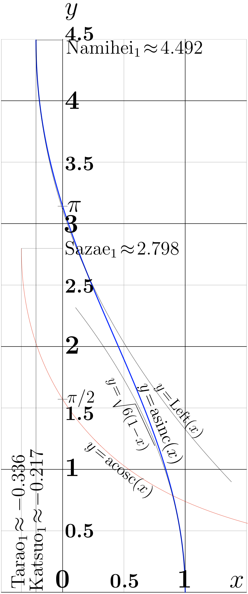
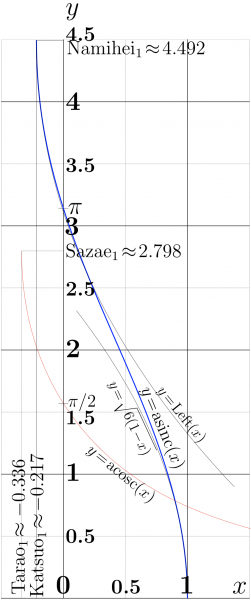
Explicit plot of functions ArcSinc (thick blue curve) and ArcCosc (thin red curve):

$y=\mathrm{asinc}(x)~$ and $~ y=\mathrm{acosc}(x)~$

For comparison, the two asymptotics of function ArcSinc are also plotted with thin black curves:

$\displaystyle y~=~ \mathrm{Left}(x)~ =~ \mathrm{Namihei} ~-~ \sqrt{\frac{-~ 2}{\mathrm{Katsuo}} (x\!-\!\mathrm{Katsuo})}

~+~ \frac{2(x\!-\!\mathrm{Katsuo})}{3~ \mathrm{Namihei}}$ that aproximates ArcSinc in cicinity of Katsuo, id est, in the left hand side of the figure, and

$y=\sqrt{6(1\!-\!x)}$

that approximates ArcSinc in vicinity of unity, id est, in the right hand side of the figure.

asinc.cin

z_type acos(z_type z){
if(Im(z)<0){if(Re(z)>=0){return I*log( z + sqrt(z*z-1.) );} 
                   else{return I*log( z - sqrt(z*z-1.) );}}
           if(Re(z)>=0){return -I*log( z + sqrt(z*z-1.) );} 
                  else {return -I*log( z - sqrt(z*z-1.) );} }

z_type asin(z_type z){
if(Im(z)<0){if(Re(z)>=0){return M_PI/2.-I*log( z + sqrt(z*z-1.) );} 
                  else {return M_PI/2.-I*log( z - sqrt(z*z-1.) );}}
          if(Re(z)>=0){return M_PI/2.+I*log( z + sqrt(z*z-1.) );} 
                 else {return M_PI/2.+I*log( z - sqrt(z*z-1.) );} }

z_type sinc(z_type z){ DB x=Re(z); DB y=Im(z); if(x*x+y*y>.01) return sin(z)/z;
z*=z; return 1.+z*(-1./6.+z*(1./120.+z*(-1./5040+z*(1./362880.))));  }

z_type sincp(z_type z){ DB x=Re(z); DB y=Im(z); z_type c; 
if(x*x+y*y>.01) return (cos(z)-sinc(z))/z;
c=z*z; return z*(-1./3.+c*(1./30.+c*(-1./840.+c*(1./45630+c*(-1./399168.))))); }

DB Namihei=4.493409457909062;
DB Katsuo=-0.21723362821122164;
z_type asincL(z_type z){int n; z_type s=Namihei-sqrt((-2./Katsuo)*(z-Katsuo));
DO(n,6)s+=(z-sinc(s))/sincp(s);  return s;}

z_type asincU(z_type z){int n; z_type s=1.4*acos(z);
  DO(n,6)s+=(z-sinc(s))/sincp(s);  return s;}

z_type asinc(z_type z){DB x=Re(z),y=fabs(Im(z));
    if(y<1. && x<0. && x>-2.6 ) return asincL(z);
                                return asincU(z); }

C++ generator of curves

// The asinc.cin above and acosc.cin and ado.cin
// should be loaded in the working directory in order to compile the C++ code below.

#include <math.h> 
#include <stdio.h>
#include <stdlib.h>
#define DB double 
#define DO(x,y) for(x=0;x<y;x++)
using namespace std;
#include <complex>
typedef complex<double> z_type;
#define Re(x) x.real()
#define Im(x) x.imag()
#define I z_type(0.,1.)
#include "ado.cin"
#include "asinc.cin"
#include "acosc.cin"

#define M(x,y) fprintf(o,"%6.4f %6.4f M\n",0.+x,0.+y);
#define L(x,y) fprintf(o,"%6.4f %6.4f L\n",0.+x,0.+y);
#define S(x,y) fprintf(o,"S\n",);

main(){ int j,k,m,n; DB x,y, p,q, t; z_type z,c,d;
DB Sazae= 2.798386045783887; // H
DB Tarao= -0.33650841691839534; // J
FILE *o;o=fopen("asincplot.eps","w");ado(o,220,470);
fprintf(o,"60 10 translate\n 100 100 scale\n");
for(m=0;m<2;m++){M(m,0)L(m,4.5)}
for(n=0;n<5;n++){M(-.5,n)L(1.5,n)}
fprintf(o,"2 setlinecap .004 W 0 0 0 RGB S\n");
for(m=-1;m<2;m++){M(.5+m,0)L(.5+m,4.5)}
for(n=0;n<5;n++){M(-.5,n+.5)L(1.5,n+.5)}
fprintf(o,"2 setlinecap .0008 W 0 0 0 RGB S\n");
DB D=(1.-Katsuo)/1000.;
M(Katsuo,Namihei)  DO(m,1000){x=Katsuo+D*(m+.5); y=Re(asinc(x)); L(x,y) }  L(1,0)
fprintf(o,"1 setlinejoin 1 setlinecap .008 W 0 0 1 RGB S\n");
M(Tarao,Sazae)DO(m,930){x=-.336+.002*m; y=Re(acosc(x)); L(x,y) }
fprintf(o,".002 W 1 0 0 RGB S\n");
M(1,0) DO(m,90){x=1.-0.01*(m+.5); y=sqrt(6.*(1.-x)); L(x,y);}
fprintf(o,".002 W 0 0 0 RGB S\n");
M(Katsuo,Namihei) DO(m,160){x=Katsuo+0.01*(m+.5); DB t=x-Katsuo; 
       y=Namihei-sqrt(-2./Katsuo*(x-Katsuo))+2.*(x-Katsuo)/3./Namihei ; L(x,y);}  
fprintf(o,".002 W 0 0 0 RGB S\n");
M(-.04,M_PI/2)L(.04,M_PI/2)
M(-.04,M_PI)L(.04,M_PI)
M(Katsuo,0)L(Katsuo,Namihei)L(0,Namihei)
fprintf(o,"2 setlinecap .002 W 0 0 0 RGB S\n"); 
M(Tarao,0)L(Tarao,Sazae)L(0,Sazae)
fprintf(o,"2 setlinecap .001 W 0 0 0 RGB S\n"); 
fprintf(o,"showpage\n%c%cTrailer",'%','%'); fclose(o);
     system("epstopdf asincplot.eps");
     system(    "open asincplot.pdf");
     getchar(); system("killall Preview");//for mac
}

Latex generator of labels

% File asincplot.pdf should be generated with the C++ code above in order to compile the Latex document below.

%<br> % Copyleft 2012 by Dmitrii Kouznetsov %<br> \documentclass[12pt]{article} %<br> \usepackage{geometry} %<br> \usepackage{graphicx} %<br> \usepackage{rotating} %<br> \paperwidth 406pt %<br> \paperheight 970pt %<br> \topmargin -90pt %<br> \oddsidemargin -106pt %<br> \textwidth 500pt %<br> \textheight 990pt %<br> \pagestyle {empty} %<br> \newcommand \sx {\scalebox} %<br> \newcommand \rot {\begin{rotate}} %<br> \newcommand \ero {\end{rotate}} %<br> \newcommand \ing {\includegraphics} %<br> \begin{document} %<br> \parindent 0pt \sx{2}{ \begin{picture}(430,490) %<br> %\put(4,6){\ing{acosplot}} %<br> % \put(4,6){\ing{aciplot}} %<br> % \put(4,6){\ing{cohcplot}} %<br> %\put(4,6){\ing{sazaecon}} %<br> \put(4,6){\ing{asincplot}} %<br> \put(66,488){\sx{1.8}{$y$}} %<br> \put(66,467){\sx{1.4}{\bf 4.5}} %<br> \put(67,456){\sx{1.3}{\rot{0}$\rm Namihei_1\!\approx\! 4.492$\ero}} %<br> \put(66,411){\sx{1.8}{\bf 4}} %<br> \put(66,361){\sx{1.4}{\bf 3.5}} %<br> \put(68,327){\sx{1.7}{$\pi$}} %<br> \put(65,310){\sx{1.8}{\bf 3}} %<br> \put(66,292){\sx{1.3}{\rot{0}$\rm Sazae_1\!\approx \!2.798$\ero}} %<br> \put(66,261){\sx{1.4}{\bf 2.5}} %<br> \put(66,211){\sx{1.8}{\bf 2}} %<br> \put(68,171){\sx{1.2}{$\pi/2$}} %<br> \put(66,157){\sx{1.4}{\bf 1.5}} %<br> \put(66,111){\sx{1.8}{\bf 1}} %<br> \put(66, 61){\sx{1.4}{\bf 0.5}} %<br> \put(33,19){\sx{1.3}{\rot{90}$\rm Tarao_1\!\approx -0.336$\ero}} %<br>\put(58, 20){\sx{1.7}{\bf 0}} %<br> \put(48,17){\sx{1.3}{\rot{90}$\rm Katsuo_1\!\approx \!-0.217$\ero}} %<br>\put(58, 20){\sx{1.7}{\bf 0}} %<br> \put( 58, 20){\sx{1.8}{\bf 0}} %<br> \put(103, 20){\sx{1.4}{\bf 0.5}} %<br> \put(201, 20){\sx{1.8}{$x$}} %<br> \put(158, 20){\sx{1.8}{\bf 1}} %<br> %\put(130, 210){\sx{.9}{\rot{-53}$y\!=\! \mathrm{Namihei}-\sqrt{2(\mathrm{Katsuo}\!+\!x)}$\ero}} %<br> \put(140, 184){\sx{1.01}{\rot{-51}$y\!=\! \mathrm{Left}(x)$\ero}} %<br> \put(127, 185){\sx{1.2}{\rot{-67}$y\!=\!\mathrm{asinc}(x)$\ero}} %<br> \put(101, 190){\sx{0.99}{\rot{-65}$y\!=\!\sqrt{6(1\!-\!x)}$\ero}} %<br> \put(83,135){\sx{1.1}{\rot{-39}$y\!=\!\mathrm{acosc}(x)$\ero}} %<br> \end{picture} %<br> } %<br> \end{document} %

Referrences

Keywords

ArcSinc