File:DoyaplotTc.png

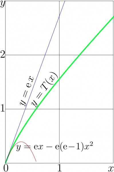
Doya function with parameter unity of real argument, $y=T(x)=\mathrm{Doya}_1(x)$ is shown with thick green line.

The linear approximation in vicinity of zero $y=T'(0) x =\mathrm e x~$ is shown with thin blue line.

The quadratic approximation in vicinity of zero $y=T'(0) x +\frac{1}{2}T(0)x^2 =\mathrm e x - \mathrm e (\mathrm e\!-\!1)x^2$ is shown with thin blue line.

Generator of curves

// Files doya.cin and ado.cin should be loaded in the working directory in order to compile the code below:

#include <math.h>
#include <stdio.h>
#include <stdlib.h>
#define DB double
#define DO(x,y) for(x=0;x<y;x++)
using namespace std;
#include <complex>
typedef complex<double> z_type;
#define Re(x) x.real()
#define Im(x) x.imag()
#define I z_type(0.,1.)
DB ArcTania(DB x){ return x+log(x)-1.;}
#include "ado.cin"
#include "doya.cin"
#define M(x,y) fprintf(o,"%7.4f %7.4f M\n",0.+x,0.+y);
#define L(x,y) fprintf(o,"%7.4f %7.4f L\n",0.+x,0.+y);
main(){ int j,k,m,n; DB x,y,t,e, a; z_type z;
FILE *o;o=fopen("doyaplot1.eps","w");ado(o,208,308);
fprintf(o,"4 4 translate\n 100 100 scale\n");
fprintf(o,"2 setlinecap\n");
for(m=0;m<3;m++){ M(m,0)L(m,3)}
for(n=0;n<4;n++){ M(0,n)L(2,n)}   
fprintf(o,".004 W 0 0 0 RGB S\n");
fprintf(o,"2 setlinejoin 1 setlinecap\n");
M(0,0);  for(n=1;n<151;n++){x=.02*n;z=x;y=Re(Doya(1.,z)); L(x,y)}
fprintf(o,".02 W 0 1 0 RGB S\n");
M(0,0); for(n=1;n<58;n++){x=.01*n; y=M_E*x*(1.-x*(M_E-1.))  ; L(x,y)}
fprintf(o,".005 W .8 0 0 RGB S\n");
M(0,0) L(3./M_E,3.)  fprintf(o,".005 W 0 0 .8 RGB S\n");
//M(0,0); for(n=0;n<110;n++){x=.01+.01*n; y=M_E*x*(1.+x*(1.-M_E + x*(.5+M_E*(-2.+M_E*1.5))))  ; L(x,y)}
fprintf(o,"showpage\n%cTrailer",'%'); fclose(o);
system("epstopdf doyaplot1.eps");
system(    "open doyaplot1.pdf"); //these 2 commands may be specific for macintosh
getchar(); system("killall Preview");// if run at another operational sysetm, may need to modify
}

Generator of labels

% File doyaplot1.pdf should be generated with the code above in order to compile the Latex document below:

% <br> \documentclass[12pt]{article} %<br> \usepackage{geometry} %<br> \usepackage{graphicx} %<br> \usepackage{hyperref} %<br> \usepackage{rotating} %<br> \usepackage{color} %<br> \definecolor{red}{rgb}{1,0.1,0.1} %<br> \definecolor{black}{rgb}{0,0,0} %<br> \definecolor{white}{rgb}{1,1,1} %<br> \definecolor{yellow}{rgb}{1,.93,0} %<br> \definecolor{bluedark}{rgb}{0,0,.87} %<br> \paperwidth 424pt %<br> \paperheight 638pt %<br> \topmargin -96pt %<br> \oddsidemargin -68pt %<br> \textwidth 1224pt %<br> \textheight 1470pt %<br> %<br> \newcommand \sx {\scalebox} %<br> \newcommand \ing {\includegraphics} %<br> \newcommand \tet {\mathrm{tet}} %<br> \newcommand \pen {\mathrm{pen}} %<br> \newcommand \bC {\mathbb C} %<br> \newcommand \rme {\mathrm e} %<br> \newcommand \rmi {\mathrm i} %<br> \newcommand \ds {\displaystyle} %<br> \newcommand \rot {\begin{rotate}} %<br> \newcommand \ero {\end{rotate}} %<br> \begin{document} %<br> \parindent 0pt %<br> \normalsize %<br> \sx{2}{ %<br> \begin{picture}(200,300) %<br> \put(0,0){\ing{doyaplot1}} %<br> \put(-6,297){\sx{1.7}{$y$}} %<br> %\put(-36,300){\sx{1.7}{$T(z)$}} %<br> \put(-6,200){\sx{1.7}{$2$}} %<br> \put(-6,100){\sx{1.7}{$1$}} %<br> \put(0,-11){\sx{1.7}{0}} %<br> \put(100,-11){\sx{1.7}{1}} %<br> \put(195,-11){\sx{1.7}{$x$}} %<br> %<br> \put( 38,110){\rot{70}{\sx{1.6}{$y=\mathrm e\, x$}}\ero} %<br> \put( 58,109){\rot{54}{\sx{1.6}{$y=T(x)$}}\ero} %<br> \put( 24,30){\sx{1.5}{$y=\mathrm e x - \mathrm e (\mathrm e\!-\!1) x^2$}} %<br> \end{picture}} %<br> \end{document} %<br> %