File:SincplotT.png

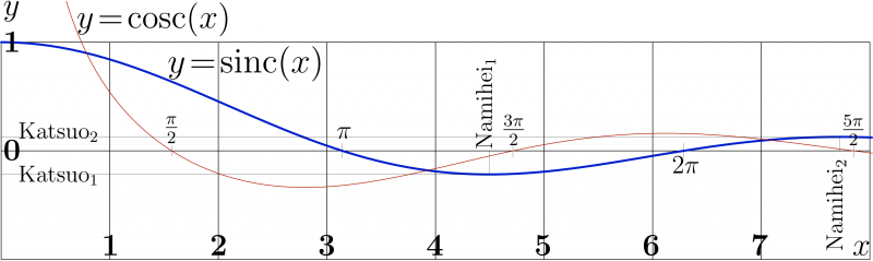
Plotof finction sinc (thick blue curve) and that of cosc.

C++ generator of curves

// File ado.cin should be loaded in the working directory in order to compile the C++ code below.

//(Warning: numeration of positive extrema begins with zero! it was not a good idea, but in the code it is so..)

#include <math.h> 
#include <stdio.h>
#include <stdlib.h>
#define DB double 
#define DO(x,y) for(x=0;x<y;x++)
using namespace std;
#include <complex>
typedef complex<double> z_type;
#define Re(x) x.real()
#define Im(x) x.imag()
#define I z_type(0.,1.)
#include "ado.cin"
#define M(x,y) fprintf(o,"%6.4f %6.4f M\n",0.+x,0.+y);
#define L(x,y) fprintf(o,"%6.4f %6.4f L\n",0.+x,0.+y);
#define S(x,y) fprintf(o,"S\n",);
main(){ int j,k,m,n; DB x,y, p,q, t; z_type z,c,d;
//DB y1 = 1.1996786402577337;
DB Sazae  = 2.798386045783887;
DB Tarao  =-0.33650841691839534;
DB Ho     =1.199678640257734;
DB Fune   =1.199678640257734;
DB Wakame =1.50887956153832;
DB Namihei= 4.493409457909062;
DB Katsuo =-0.21723362821122164;
DB Namihei1=7.725251836937619; 
DB Katsuo1 =0.12837455352589913;
FILE *o;o=fopen("sincplot.eps","w");ado(o,820,250);
fprintf(o,"10 110 translate\n 100 100 scale\n");
for(m=0;m<9;m++){M(m,-1)L(m,1)}
for(n=-1;n<2;n++){M(0,n)L(8,n)}
fprintf(o,"2 setlinecap .006 W 0 0 0 RGB S\n"); 
// DO(m,291){ x=.336+.01*m; y=cosh(x)/x; if(m==0)M(x,y) else L(x,y) }
// fprintf(o,"1 setlinejoin 1 setlinecap .02 W 0 .8 0 RGB S\n");
M(0,1); DO(m,81){ x=.1*(m+.5); y=sin(x)/x; L(x,y) }
fprintf(o,"1 setlinejoin 1 setlinecap .02 W 0 0 .8 RGB S\n");
//M(Fune,0)L(Fune,Wakame)L(0,Wakame) fprintf(o,"2 setlinecap .003 W 0 0 0 RGB S\n");
//DO(m,476){ x=.31+.01*m;  y=cos(x)/x;
DO(m,750){ x=.6+.0101*m;  y=cos(x)/x;  if(m==0)M(x,y) else L(x,y) }
fprintf(o,"1 setlinejoin 1 setlinecap .006 W .8 0 0 RGB S\n"); p=1.8;q=.7;
M(Namihei,0)L(Namihei,Katsuo)L(0,Katsuo)
M(Namihei1,0)L(Namihei1,Katsuo1)L(0,Katsuo1)
//M(Sazae,0)L(Sazae,Tarao)L(0,Tarao) 
M(.5*M_PI,-.05)L(.5*M_PI,.05)
M(1.5*M_PI,-.06)L(1.5*M_PI,.05)
M(2.5*M_PI,-.06)L(2.5*M_PI,.05)
M( M_PI,-.07)L( M_PI,.07) M(2*M_PI,-.07)L(2*M_PI,.07)
fprintf(o,"2 setlinecap .002 W 0 0 0 RGB S\n");
fprintf(o,"showpage\n%c%cTrailer",'%','%'); fclose(o);
    system("epstopdf sincplot.eps");
    system(    "open sincplot.pdf");
    getchar(); system("killall Preview");//for mac
}

Latex generator of labels

%File sincplot.pdf should be generated with the code above %(and stored in the working directory) %in order to compile the Latex document below.

%<br> % Copyleft 2012 by Dmitrii Kouznetsov %<br> \documentclass[12pt]{article} %<br> \usepackage{geometry} %<br> \usepackage{graphicx} %<br> \usepackage{rotating} %<br> \paperwidth 1614pt %<br> \paperheight 482pt %<br> \topmargin -90pt %<br> \oddsidemargin -106pt %<br> \textwidth 900pt %<br> \textheight 900pt %<br> \pagestyle {empty} %<br> \newcommand \sx {\scalebox} %<br> \newcommand \rot {\begin{rotate}} %<br> \newcommand \ero {\end{rotate}} %<br> \newcommand \ing {\includegraphics} %<br> \begin{document} %<br> \parindent 0pt \sx{2}{ \begin{picture}(830,246) %<br> %\put(4,6){\ing{acosplot}} %<br> % \put(4,6){\ing{aciplot}} %<br> % \put(4,6){\ing{cohcplot}} %<br> %\put(4,6){\ing{sazaecon}} %<br> \put(4,6){\ing{sincplot}} %<br> \put(16,242){\sx{2.5}{$y$}} %<br> %\put(16,309){\sx{2.2}{\bf 2}} %<br> \put(16,208){\sx{2.4}{\bf 1}} %<br> %\put(16,160){\sx{1.8}{\bf 2.5}} %<br> %\put(16, 262){\sx{2.2}{Wakame}} %<br> \put(16,108){\sx{2.4}{\bf 0}} %<br> %\put(16, 75){\sx{2.4}{Tarao}} %<br> \put(30, 128){\sx{1.8}{$\rm Katsuo_2$}} %<br> \put(30, 88){\sx{1.8}{$\rm Katsuo_1$}} %<br> \put(107, 20){\sx{2.4}{\bf 1}} %<br> %\put(142,120){\sx{2.4}{\rot{90}Fune\ero}} %<br> \put(207, 20){\sx{2.4}{\bf 2}} %<br> %\put(302,118){\sx{2.5}{\rot{90}Sazae\ero}} %<br> \put(468,118){\sx{1.8}{\rot{90}$\rm Namihei_1$\ero}} %<br> \put(792, 24){\sx{1.8}{\rot{90}$\rm Namihei_2$\ero}} %<br> \put(307, 20){\sx{2.4}{\bf 3}} %<br> \put(407, 20){\sx{2.4}{\bf 4}} %<br> \put(507, 20){\sx{2.4}{\bf 5}} %<br> \put(607, 20){\sx{2.4}{\bf 6}} %<br> \put(707, 20){\sx{2.4}{\bf 7}} %<br> %\put(807, 20){\sx{2.2}{\bf 8}} %<br> \put(164, 132){\sx{2}{$\frac{\pi}{2}$}} %<br> \put(324, 128){\sx{2}{$\pi$}} %<br> \put(476, 130){\sx{2}{$\frac{3\pi}{2}$}} %<br> \put(634, 96){\sx{2}{$2\pi$}} %<br> \put(790, 130){\sx{2}{$\frac{5\pi}{2}$}} %<br> \put(801, 20){\sx{2.5}{$x$}} %<br> \put( 84, 230){\sx{2.6}{\rot{0}$y\!=\!\mathrm{cosc}(x)$\ero}} %<br> \put(168, 189){\sx{2.7}{\rot{0}$y\!=\!\mathrm{sinc}(x)$\ero}} %<br> \end{picture} %<br> } %<br> \end{document} %

References