File:AcoscplotT.png

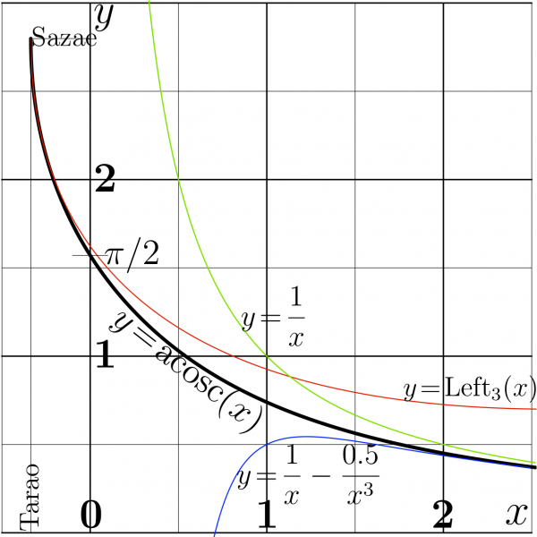
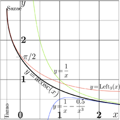
Explicit plot of function ArcCosc=acosc and its asymptotics.

$\mathrm{cosc}(\mathrm{Sazae})=\mathrm{Tarao}$

$\mathrm{cosc}'(\mathrm{Sazae})=0$

$\mathrm{Sazae} \approx ~ 2.798386045783887$

$\mathrm{Tarao} \approx\! -0.33650841691839534$

$\mathrm{acosc}(\mathrm{Tarao})=\mathrm{Sazae}$

$\displaystyle \mathrm{Left}_3(z)=\mathrm{Sazae}

- \sqrt{

           \frac{2(z-\mathrm{Tarao})}
                   {- \mathrm{Tarao} }} 

- \frac{2 (z -\mathrm{Tarao})}

          {3 ~\rm  Sazae~Tarao} $

C++ Implementation of acosc

The text below should be stored in the working directory as acosc.cin.

z_type cosc(z_type z) {return cos(z)/z;}
z_type cosp(z_type z) {return (-sin(z) - cos(z)/z)/z ;}
z_type cohc(z_type z) {return cosh(z)/z ;}
z_type cohp(z_type z) {return (sinh(z)-cosh(z)/z)/z ;}

z_type acoscL(z_type z){ int n; z_type s,q; z*=-I; q=I*sqrt(1.50887956153832-z);
  s=q*1.1512978931181814 + 1.199678640257734; DO(n,6) s+= (z-cohc(s))/cohp(s);
  return -I*s; }

z_type acoscR(z_type z) {int n; z_type s= (1.-0.5/(z*z))/z;
       DO(n,5) s+=(z-cosc(s))/cosp(s); return s;}

z_type acoscB(z_type z){ z_type t=0.33650841691839534+z, u=sqrt(t), s; int n;
s=    2.798386045783887
+u*(-2.437906425896532
+u*( 0.7079542331649882 
+u*(-0.5009330133042798
+u*( 0.5714459932734446    ))));
DO(n,6) s+=(z-cosc(s))/cosp(s); return s; }

z_type acosc(z_type z){ DB x1=-0.33650841691839534, x=Re(z), y=Im(z), yy=y*y, 
r=x-x1;r*=r;r+=yy; if(r < 1.8 )     return acoscB(z); 
r=x+2.;r*=r;r+=yy; if(r>8. && x>=0) return acoscR(z);
if(y >= 0) return acoscL(z);
      return conj(acoscL(conj(z))); }

C++ generator of curves

The acosc.cin above and ado.cin should be loaded in the working directory in order to compile the C++ code below.

#include <math.h> 
#include <stdio.h>
#include <stdlib.h>
#define DB double 
#define DO(x,y) for(x=0;x<y;x++)
using namespace std;
#include <complex>
typedef complex<double> z_type;
#define Re(x) x.real()
#define Im(x) x.imag()
#define I z_type(0.,1.)
#include "ado.cin"
#include "acosc.cin"

#define M(x,y) fprintf(o,"%6.4f %6.4f M\n",0.+x,0.+y);
#define L(x,y) fprintf(o,"%6.4f %6.4f L\n",0.+x,0.+y);
#define S(x,y) fprintf(o,"S\n",);

main(){ int j,k,m,n; DB x,y, p,q, t; z_type z,c,d;
DB Sazae= 2.798386045783887; // H
DB Tarao= -0.33650841691839534; // J
FILE *o;o=fopen("acosplot.eps","w");ado(o,320,330);
fprintf(o,"60 10 translate\n 100 100 scale\n");
for(m=0;m<4;m++){M(m,0)L(m,3)}
for(n=0;n<4;n++){M(-.5,n)L(2.5,n)}
fprintf(o,"2 setlinecap .008 W 0 0 0 RGB S\n");
for(m=-1;m<3;m++){M(.5+m,0)L(.5+m,3)}
for(n=0;n<4;n++){M(-.5,n+.5)L(2.5,n+.5)}
fprintf(o,"2 setlinecap .003 W 0 0 0 RGB S\n");
M(Tarao,Sazae)DO(m,1430){x=-.336+.002*m; y=Re(acosc(x)); L(x,y) }
fprintf(o,"1 setlinejoin 1 setlinecap .02 W 0 0 0 RGB S\n");
M(Tarao,Sazae)DO(m,1430){x=-.33+.002*m; z=x; 
y=Sazae - (sqrt((-2./Tarao)*(x-Tarao))+2./(3.*Sazae*Tarao)*(x-Tarao) ) ; L(x,y);}
fprintf(o,"1 setlinejoin 1 setlinecap .005 W 1 0 0 RGB S\n");
DO(m,220){x=.33+.01*m;
y=1./x ; if(m==0)M(x,y) else L(x,y)}
fprintf(o,"1 setlinejoin 1 setlinecap .005 W 0 1 0 RGB S\n");
DO(m,180){x=.7+.01*m;
y=1./x*(1.-.5/(x*x)) ; if(m==0)M(x,y) else L(x,y)}
fprintf(o,"1 setlinejoin 1 setlinecap .005 W 0 0 1 RGB S\n");
M(-.1,M_PI/2)L(.1,M_PI/2)
M(Tarao,0)L(Tarao,Sazae)L(0,Sazae)
fprintf(o,"2 setlinecap .003 W 0 0 0 RGB S\n"); 
fprintf(o,"showpage\n%c%cTrailer",'%','%'); fclose(o);
     system("epstopdf acosplot.eps");
     system(    "open acosplot.pdf");
     getchar(); system("killall Preview");//for mac
}

Latex generator of labels

FIe acosplot.pdf should be generated with the code above in order to complile the Latex document below. In order to avoid confusion with acosplot.pdf, the docuemnt below is recommended to store as acoscplotT.tex

% % Copyleft 2012 by Dmitrii Kouznetsov %<br> \documentclass[12pt]{article} %<br> \usepackage{geometry} %<br> \usepackage{graphicx} %<br> \usepackage{rotating} %<br> \paperwidth 610pt %<br> \paperheight 610pt %<br> \topmargin -92pt %<br> \oddsidemargin -106pt %<br> \textwidth 900pt %<br> \textheight 900pt %<br> \pagestyle {empty} %<br> \newcommand \sx {\scalebox} %<br> \newcommand \rot {\begin{rotate}} %<br> \newcommand \ero {\end{rotate}} %<br> \newcommand \ing {\includegraphics} %<br> \newcommand \ds {\displaystyle} %<br> \begin{document} %<br> \parindent 0pt \sx{2}{ \begin{picture}(340,310) %<br> \put(4,6){\ing{acoscplot}} %<br> %\put(4,6){\ing{aciplot}} %<br> \put(66,306){\sx{2}{$y$}} %<br> %\put(42,290){\sx{2}{$f_0$}} %<br> \put(33,292){\sx{1.6}{Sazae}} %<br> \put(66,210){\sx{2}{\bf 2}} %<br> \put(72,169){\sx{1.7}{$\pi/2$}} %<br> \put(66,110){\sx{2}{\bf 1}} %<br> %\put(21, 21){\sx{2.1}{$z_0$}} %<br> \put(36, 17){\sx{1.6}{\rot{90}Tarao\ero}} %<br> \put(58, 19){\sx{2}{\bf 0}} %<br> \put(158, 19){\sx{2}{\bf 1}} %<br> \put(258, 19){\sx{2}{\bf 2}} %<br> \put(300, 21){\sx{2.1}{$x$}} %<br> %\put(110,238){\sx{1.4}{\rot{0}$\ds y\!=\!\frac{1}{x}$\ero}} %<br> \put(150,134){\sx{1.4}{\rot{0}$\ds y\!=\!\frac{1}{x}$\ero}} %<br> \put(237,94){\sx{1.3}{ $\ds y\!=\! \mathrm{Left}_3(x)$}} %<br> \put(142,46){\sx{1.3}{ $\ds y\!=\! \frac{1}{x}-\frac{0.5}{x^3}$}} %<br> %\put(168,94){\sx{1.6}{\rot{-16}$y\!=\!\mathrm{acosc}(x)$\ero}} %<br> \put(76,134){\sx{1.7}{\rot{-36}$y\!=\!\mathrm{acosc}(x)$\ero}} %<br> \end{picture} %<br> } %<br> \end{document} %

Conversion

The acoscplotT.pdf generated with the code above is converted to the PNG format with default resolution 150 pix/inch.