File:AcosqqplotT.png

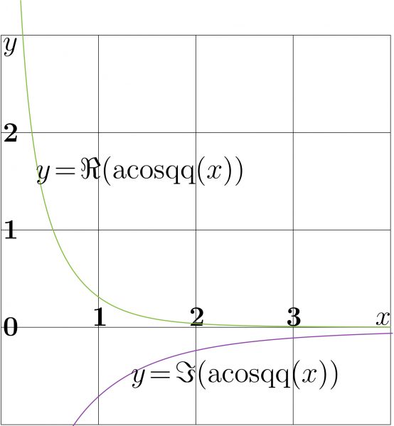
Graphic of function ArcCosqq (or acosqq) defined with

$\text{acosqq}(z)=\text{acosq}(z)\, \tan\!\!\big( \text{acosq}(z) \big)$

through functions acosq (or ArcCosq); it is expressed as;

$\text{acosq}(z)=\text{acosq}\big( \mathrm e ^{\mathrm i \pi /4}\, z \big)$

which is ArcCosc of argument rotated for the phase quarter of $\pi$. Namely this phase appear in the application for the atom optics, for channelling of particle between absorbing walls.

acosc or ArcCosc is inverse funciotn of cosc,

$\displaystyle \text{cosc}(z)=\frac{\cos(z)}{z}$

Use of function acosqq

acoscqq expresses the decay constant of mode guided between absorbing waves, see the special article Absorbing Schroedinger for the details.

C++ generator of curves

Files ado.cin and acosc.cin should be loaded into the working directory in order to compile the C++

#include <math.h> 
#include <stdio.h>
#include <stdlib.h>
#define DB double 
#define DO(x,y) for(x=0;x<y;x++)
using namespace std;
#include <complex>
typedef complex<double> z_type;
#define Re(x) x.real()
#define Im(x) x.imag()
#define I z_type(0.,1.)

#include "ado.cin"

#include "acosc.cin"

z_type acosq(z_type z){ z_type c=z*exp(I*M_PI/4.); c=acosc(c); return c;}

z_type acosqq(z_type z){ z_type c=z*exp(I*M_PI/4.); c=acosc(c); return c*tan(c);}

#define M(x,y) fprintf(o,"%6.4f %6.4f M\n",0.+x,0.+y);
#define L(x,y) fprintf(o,"%6.4f %6.4f L\n",0.+x,0.+y);
#define S(x,y) fprintf(o,"S\n",);
main(){ int j,k,m,n; DB x,y, p,q, t; z_type z,c,d;
DB Sazae= 2.798386045783887; // H
DB Tarao= -0.33650841691839534; // J
FILE *o;o=fopen("acosqqplot.eps","w");ado(o,420,460);
fprintf(o,"10 110 translate\n 100 100 scale\n");
for(m=0;m<5;m++){M(m,-1)L(m,3)}
for(n=-1;n<4;n++){M(0,n)L(4,n)}
fprintf(o,"2 setlinecap .005 W 0 0 0 RGB S\n");
/*
for(m=-4;m<3;m++){M(.5+m,-1)L(.5+m,3)}
for(n=-1;n<3;n++){M(-4,n+.5)L(4,n+.5)}
fprintf(o,"2 setlinecap .003 W 0 0 0 RGB S\n");
*/
DO(m,381){x=0.198+.01*m;  y=Re(acosqq(x)); if(m==0)M(x,y)else L(x,y);
       printf("%6.3f %6.3f\n",x,y); }
fprintf(o,"1 setlinejoin 1 setlinecap .011 W 0 .6 0 RGB S\n");
DO(m,330){x=0.73+.01*m; y=Im(acosqq(x)); if(m==0)M(x,y)else L(x,y) }
fprintf(o,"1 setlinejoin 1 setlinecap .01 W .7 0 .7 RGB S\n");
// M(-.1,M_PI/2)L( .1,M_PI/2)  fprintf(o,".004 W 0 0 0 RGB S\n");
fprintf(o,"showpage\n%c%cTrailer",'%','%'); fclose(o);
     system("epstopdf acosqqplot.eps");
     system(    "open acosqqplot.pdf");
     getchar(); system("killall Preview");//for mac
}

Latex generator of labels

File acosqqplot.pdf should be generated with the code above in order to compile the Latex document below.

%<br> % Copyleft 2012 by Dmitrii Kouznetsov %<br> \documentclass[12pt]{article} %<br> \usepackage{geometry} %<br> \usepackage{graphicx} %<br> \usepackage{rotating} %<br> \paperwidth 812pt %<br> \paperheight 878pt %<br> \topmargin -90pt %<br> \oddsidemargin -106pt %<br> \textwidth 900pt %<br> \textheight 900pt %<br> \pagestyle {empty} %<br> \newcommand \sx {\scalebox} %<br> \newcommand \rot {\begin{rotate}} %<br> \newcommand \ero {\end{rotate}} %<br> \newcommand \ing {\includegraphics} %<br> \begin{document} %<br> \parindent 0pt \sx{2}{ \begin{picture}(140,444) %<br> %\put(4,6){\ing{sazaecon}} %<br> \put(16,402){\sx{2.5}{$y$}} %<br> \put(16,308){\sx{2.4}{\bf 2}} %<br> %\put(422,269){\sx{2.4}{$\pi/2$}} %<br> \put(16,208){\sx{2.4}{\bf 1}} %<br> %\put(16, 262){\sx{2.2}{Wakame}} %<br> \put(16,108){\sx{2.4}{\bf 0}} %<br> %\put(16, 75){\sx{2.4}{Tarao}} %<br> %\put(200, 118){\sx{2.4}{\bf -2}} %<br> %\put(300, 118){\sx{2.4}{\bf -1}} %<br> \put(108, 118){\sx{2.4}{\bf 1}} %<br> %\put(142,120){\sx{2.4}{\rot{90}Fune\ero}} %<br> \put(208, 118){\sx{2.4}{\bf 2}} %<br> %\put(302,118){\sx{2.5}{\rot{90}Sazae\ero}} %<br> \put(308, 118){\sx{2.4}{\bf 3}} %<br> %\put(807, 120){\sx{2.2}{\bf 4}} %<br> %\put(161, 132){\sx{2.8}{$\frac{\pi}{2}$}} %<br> %\put(471, 130){\sx{2.6}{$\frac{3\pi}{2}$}} %<br> \put(400, 119){\sx{2.4}{$x$}} %<br> \put(4,6){\ing{acosqqplot}} %<br> \put(50,270){\sx{2.52}{\rot{0}$y\!=\!\Re(\mathrm{acosqq}(x))$\ero}} %<br> \put(148, 60){\sx{2.52}{\rot{0}$y\!=\!\Im(\mathrm{acosqq}(x))$\ero}} %<br> \end{picture} %<br> } %<br> \end{document} %