Discrete Bessel

Discrete Bessel is one of the discrete approximations of the Bessel transform.

This article describes the simple implementation in Mathematica language and the testing.

Bessel transform

Let the Bessel transform \(f\) of function \(g\) be defined with

\(\displaystyle f(x)=\int_0^\infty J_v(xy)\, g(y)\, y\, \mathrm d y \)

where \(J_v\) is the Bessel function of order \(v\). Often, \(v\) is assumed to be integer number or just zero.

Here \(x\) may have sense of the radial coordinate (in polar system of coordinates), measured in some appropriate units; then \(y\) has sense of the corresponding radial wavenumber.

Such a representation takes 21 symbols and seems to be simplest possible.

Naive implementation

This section represents the Mathematica implementation and its test.

Example with \(~M\!=\!8\)

M = 8;
S = 1. BesselJZero[0, M+1];
X[n_] = BesselJZero[0,n]/Sqrt[S];
W[n_] = Sqrt[2./S]/Abs[BesselJ[1, BesselJZero[0,n]]];
T = Table[Table[W[m] BesselJ[0, X[m] X[n]] W[n], {n,1,M}], {m,1,M}];
Id = IdentityMatrix[M];
TT = T.T;
TableForm[Table[{X[n], W[n]}, {n,1,M}]]
TableForm[T]
TableForm[TT]

This code produces the output; it begins with table of 8 coordinates \(x\) of the grid points and the corresponding weights \(w\) :

\(\begin{array}{ll} 0.4586366203331863 &0.5195285071552199\\ 1.0527624177874753 & 0.7926530133638695\\ 1.650396849184917 & 0.9935886501287517\\ 2.2488240306434886 &1.1602517418890865\\ 2.8475519209198557 & 1.3058173905056825\\ 3.446425324924121 & 1.4367104029426196\\ 4.0453800503454875 & 1.556635975360147\\ 4.644384788693245 & 1.6679612725451483 \end{array}\)

In this approximation

\( f_n=f(x_n) \, w_n \)
\( g_n=g(x_n) \, w_n \)

\( \displaystyle f_m \approx \sum_{n=1}^M T_{m,n} \, g_n \)

\( \displaystyle g_m \approx \sum_{n=1}^M T_{m,n} \, f_n \)

Matrix \(T\) is symmetric and almost unitary; \(T\!\approx\! T^{-1}\).

For \(M\!=\!8\), the deviation of \(T^2\) from the identity matrix is of order of \(10^{-7}\). This deviation quickly drops at the increasing of number \(M\) of the nodes.

At the grid, the scalar product of two functions \(\phi\) and \(\psi\) is approximated with

\(\phi^{\dagger} \psi=\,\) \(\displaystyle \displaystyle \int_0^\infty \phi(r)^*\, \psi(r)\, r\, \mathrm dr \approx\,\) \(\displaystyle \sum_{n=1}^M \, \phi_n^*\, \psi_n=\,\) \(\displaystyle \sum_{n=1}^M \, \phi(x_n)^*\, \psi(x_n)\, {w_n}{^2}\)

Test with the eigenfunction

The Bessel function transform has eigenfunctions; they are self–bessels: such a function is Bessel transform is itself.

Simplest among these functions is Gaussian, \(f(x)=\exp(-x^2/2)\).

For the coordinates X, weights W and matrix \(T\), calculated in the example 1, the test can be written as follows:

F = Table[{Exp[-X[n]^2/2] W[n]}, {n, 1, M}]
T.F

The test prints two almost identical lines,

{{0.467663}, {0.455425}, {0.25453}, {0.0925536}, {0.0226534}, {0.00378554}, {0.000435062}, {0.0000345345}}

{{0.467663}, {0.455425}, {0.25453}, {0.0925535}, {0.0226534}, {0.00378551}, {0.000435082}, {0.0000344505}}

The same test can be performed also in C++ with code below:

#include<math.h>
#include<stdio.h>
#define DB double
#define DO(x,y) for(x=0;x<y;x++)
DB jnp(int n,DB x){ return .5*( jn(n-1,x)-jn(n+1,x) ) ; } // Derivative of n th Bessel
DB jnz(int v, int k){ DB x,t; t=M_PI*(k+.5*v-.25); x= t - (v*v-.25)*.5/t;
                x-= jn(v,x)/jnp(v,x); // Newton adjustment of the root
                x-= jn(v,x)/jnp(v,x);
                x-= jn(v,x)/jnp(v,x);
                return x; } // the k th zero of v th Bessel

int main(){ int m,n,v,k; DB s, x,y; int M=8;
DB X[M+1],W[M+1],T[M+1][M+1],TT[M+1][M+1], F[M],G[M];
DB S=jnz(0,M+1);
DB qs=sqrt(1./S);
DB q=sqrt(2./S);
for(n=1;n<M+1;n++){ x=jnz(0,n); X[n]=x*qs; y=W[n]=q/fabs(j1(x));
                        printf("%3d %20.16lf %20.16lf\n",n,X[n],W[n]); }
for(m=1;m<=M;m++){ printf("%2d",m); for(n=1;n<=M;n++){ T[m][n]=W[m]*j0(X[m]*X[n])*W[n]; }}
for(m=1;m<=M;m++){printf("\n"); for(n=1;n<=M;n++){printf("%14.10lf",T[m][n]); }}
printf("\n");
for(m=1;m<=M;m++){printf("\n");
for(n=1;n<=M;n++){s=0.; for(k=1;k<=M;k++) s+=T[m][k]*T[k][n] ;
                        TT[m][n]=s;printf("%14.10lf",TT[m][n]); }}
printf("\n\n");
for(m=1;m<=M;m++){x=X[m]; y=exp(-x*x/2.); F[m]=y*W[m]; printf("%14.10lf",F[m]); }
printf("\n");
for(m=1;m<=M;m++){ s=0.; for(n=1;n<=M;n++) s+=T[m][n]*F[n]; G[m]=s; }
for(m=1;m<=M;m++) printf("%14.10lf",G[m]);
printf("\n");
return 0;}

\(y=\exp(-x^2/2)\), black solid line; the representation at nodes of the mesh, small red circles; the discrete transform, big blue curcles

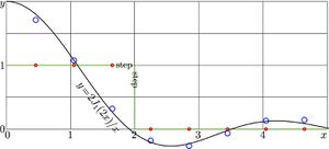
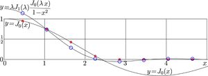
The C++ algorithm above is used in the code that generates figure at right.

The discrete Bessel on the grid of 8 nodes reproduces 7 decimal digits of the simplest self-Bessel function.

The same Gaussian is also self-Fourier, and in the similar way can be used for testing of the discrete Fourier transform.

Test with step function

\(y=\mathrm{UnitStep}(2\!-\!x)\), green line. The discrete representation, small red circles. The Discrete Bessel transform, big blue circles. The exact Bessel transform \(y\!=\!g(x)\), black line.

Another example with discrete Bessel transform of the step function is considered in the this section. Let

\(~f(x)=\mathrm{UnitStep}(2\!-\!x)\)

With the same arrays of coordinates X, corresponding weights W and kernel matrix T, as in the previous tests, the discrete Bessel can be calculated with the Mathematica code below:

F = Table[{ W[n] UnitStep[2-X[n]]}, {n, 1, M}]
T.F
G = Table[{ W[n] BesselJ[1, 2 X[n]] 2/X[n]}, {n, 1, M}]

It produces 3 lines of output:
{{0.519529}, {0.792653}, {0.993589}, {0.}, {0.}, {0.}, {0.}, {0.}}
{{0.888362}, {0.85255}, {0.316075}, {-0.208464}, {-0.342645}, {-0.0956198}, {0.204077}, {0.240501}}
{{0.93354} , {0.85489} , {0.265299}, {-0.237771}, {-0.297814}, {-0.0309065}, {0.189716}, {0.145389}}

The last two lines show some similarity, but, for the abrupt function, the agreement is worse than for the smooth function in the previous example. The last table corresponds to the exact integration,

\(\displaystyle g(x)=\int_0^2 J_0(xy) \,y \, \mathrm d y = 2 J_1(2x)/x\)

The C++ implementation becomes straightforward, as the example with self-Fourier from the previous section is considered; the C++ implementation is used to generate figure at right.

Test with truncated Bessel

\(y\!=\!J_0(x)\), \(y\!=\!g(x)\), black solid lines, and their discrete representations, colored circles

Let \(\lambda\) be the first zero of the Bessel function,

\(\lambda=\,\) BesselJZero\([0,1] \approx\, 2.404825557695773\)

sp, that \(~ J_0(\lambda)\!=\!0\,\). Let

\(f(x)=J_0(x)\,\)UnitStep\((\lambda\!-\!x)\)

The Bessel transform is

\(\displaystyle g(x)=\int_0^\infty f(y)\, J_0(xy)\, y\, \mathrm d y=\) \(\displaystyle \int_0^\lambda J_0(y)\, J_0(xy)\, y\, \mathrm d y=\) \(\displaystyle \lambda\, J_1(\lambda)\, \frac{ J_0(\lambda x) }{1\!-\!x^2}\)

Note, that the singularity (pole) in denominator of the last expression is compensated by the zero at its numerator; so, the function \(g\) has no singularities at the positive part of the real axis, and its first is

BesselJZero\([0,2]/\lambda=\,\)BesselJZero\([0,2]/\)BesselJZero\([0,1] \approx\, 2.2954172674276943\)

Keywords

Bessel function Bessel transform