


Term Duration may refer to the historic models of collapse of empires.
Here, Duration \(X\) is time between the two events:
A. Nulling: Some empire at the level of Federal Law abolishes, nullifies the separation of powers
B. Collapse: The adminitrative system is reinstalled
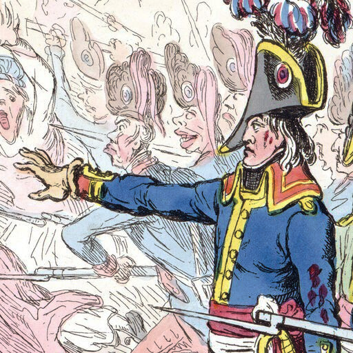
Historic cases of Nulling of separation of powers are related with historic personages shown in pictures at right.
Dates of these Nullings and dates of the following Collapses by documents
[1]
[2]
[3]
[4]
[5]
[6]
[7]
[8]
[9]
[10]
[11]
are collected in the table below.
| \(i\) | country | Nulling | Collapse | days | \(~ X_i\) , y. | refs |
| 1 | England of Cromwell | 1653.12.16 | 1661.04.23 | 2685 | 07.3513 | [1] [2] |
| 2 | France de Napoléon | 1802.08.04 | 1815.11.20 | 4856 | 13.2953 | [3] [4] |
| 3 | Italia di Mussolini | 1928.05.17 | 1947.12.27 | 7163 | 19.6116 | [5] [6] |
| 4 | Germany of Hitler | 1933.03.24 | 1945.05.08 | 4428 | 12.1235 | [7] [8] |
| 5 | Soviet Union | 1977.10.07 | 1991.08.20 | 5065 | 13.8675 | [9][10] |
| 6 | RF of putin | 2020.03.11 | 2028-2042? | 3k-7k? | 6-22 ? | [11][?] |
The first 5 rows of this table aove are used to estimate parameters of three historic models described below.
The 6th row allows the forecast for century 21 and testing the models.
This article deals with forecasts. I try to interpret them in a scientific way.
The first documented historic forecasts appear in the Bible. The Great Flood, the destruction of Sodom and Gomorrah, and other divine predictions appear in the early scripture. These stories represent not only moral or theological lessons but some of the earliest narrative models of large-scale societal collapse initiated by the corruption, lawlessness. Historically, forecasts like these are presented without revealing any reasoning behind them. The tradition is to hide the method of generation from the readers. Even when one listens carefully to a forecast by a political analyst, one cannot reconstruct the basic assumptions used to build the model, nor can one reproduce the deduction by which the prediction is derived.
The most serious forecasts of the 20th and 21st centuries include:
- «Will the Soviet Union Survive until 1984» («Просуществует ли Советский Союз до 1984 года») by Andrei Amalrik (1969) [13]
- «Moscow2042» («Москва2042») by Vladimir Voinovich (1986, Войнович Владимир Николаевич. Москва2042) [14]
- «Russia2028» by Semen Skrepetski ( «Россия2028» by Скрепецкий Семён)(2019). [15]
Even in these notable examples, the deduction is hidden from the reader.
Many other historic predictions («предсказания революций») are observed. Most of them turned out to be wrong.
Generally, forecasts in historical or political contexts are not treated as scientific concepts by academic historians, because they do not offer historic models that could be verified or refuted.
On the other hand, Editor considers History to be a science. Any science must present concepts that can be verified or rejected by future observation. This follows from the Third of the TORI axioms [16].
This version of the article presents two such models. Both are based on published historical documents whose authenticity is not in doubt. The data and calculation methods are fully transparent, allowing any colleague to independently reproduce the results.
The models below relate the separation of powers (that seems to be important achievement of the Human civilization) and collapse of those empires that exclude this achievement at the level of the Federal Law. Namely with time (Duration) between these two events in each case.
Historically, the principle of separation of powers has often led to the establishment of stable, prosperous democratic states.
Conversely, many empires have collapsed due to war, internal coups, or revolutions. Some revolutions give rise to long-lasting dictatorships - often under the facade of democracy.
There are also examples of relatively stable honest monarchies that do not pretend to be republic, but persist for centuries.
But cases in which a formally democratic state, by Federal Law, explicitly nullifies the separation of powers are rare. Only six such cases are noted (see Table near the top of this article). So far, there is no known case where the state, "republic" continued longer than 20 years after such a nulling.
In this article, we use the term «Nulling». It refers to irrecersibe change of the Federal Law, nullification of its power, transfer the functions of Law to the will of the dictator and the accomplices. The term «Nulling» is borrowed from Russian word «обнуление» that appears mainly during the 2020 constitutional amendments. No other appropriate English equivalent to refer this phenomenon is found; so, I apply this term retroactively to earlier historical events where similar legal mechanisms were used to consolidate the authority.
Here, term «nulling» denotes a formal or quasi-legal process by which a governing regime deliberately disables or cancels key institutional constraints - typically those related to the separation of powers and/or democratic oversight, providing the lifetime ruling of the current dictator. The Nulling is irreversibe. Since the Nulling, the top ruler and his/her administration cannot be replaced with civilized, constitutional way; only through the Collapse of the administrative system of the country.
Unlike a military coup, Nulling often occurs via legislative acts, constitutional amendments, or official decrees - preserving an appearance of legality while consolidating authoritarian control. It is frequently a symptom of administrative weakness, where the regime seeks to stabilize itself by eliminating internal checks.
This article attempts to generalize the observation mentioned (the Nulling is followed by the Collapse of the country, empire) into a scientific model. Three such models are constructed to describe the observed values of Duration. They deal with the first 5 examples in the table above. The sixth example is still ongoing and may serve as a test: it may confirm or refute the model(s).
The first model is based on the following postulate:
Durations for all human civilizations, societies are distributed independently and have the same Gassian (normal) distribution with some mean value \(X_0\) and some width \(\sigma_0\).
We have no ab initio model for the collapses of an empire the pretends to be democratic; so, we do not know values \(X_0\) nor that of \(\sigma_0\).
I try to extract maximal information from the empirical data.
We nave \(N\!=\!5\) completed cases in the Table 1. From the first 5 rows of the Table, I estimate the following quantities:
the sample mean \[ t=\tilde X = \frac{1}{N} \sum_{i=1}^N X_i \approx 13.2498 ~ ~\rm [years] \] The sample spread \[ s = \sqrt{ \frac{1}{N\!-\!1} \sum_{i=1}^N \left(X_i-\tilde X\right)^2 } \approx 4.3851 ~ ~ \rm [years] \] Scale for the Student distribution as the likelihood density for the sample mean \[ c = \frac{s}{\sqrt{N}} =\sqrt{ \frac{1}{N(N\!-\!1)} \sum_{i=1}^N \left(X_i-\tilde X\right)^2 } \approx 1.9611 ~ ~ \rm [years] \] I keep 4 decimal figures after a decimal point in order to simplify the tracing of the calculus; everyone performing the same calculus is supposed to get the same values. However, only first two digits in these estimates may have some predictive meaning.
Here I measure time in years. As a reminder, these units are indicated in rectangular parenthesis at each formula when the value suggested have sense of time.
For the sample with \(N\) cases, the likelihood density \(f(t)\) for \(X_0\) to have value \(t\) is
expressed through the Student Distribution with \(N\!-\!1\) degrees of freedom:
\[
f(x)= \frac{1}{c} \mathrm{Student}_{N-1}\!\left(
\frac{x-\tilde X}{c}
\right)
\]
This function is shown in figure below with red curve.
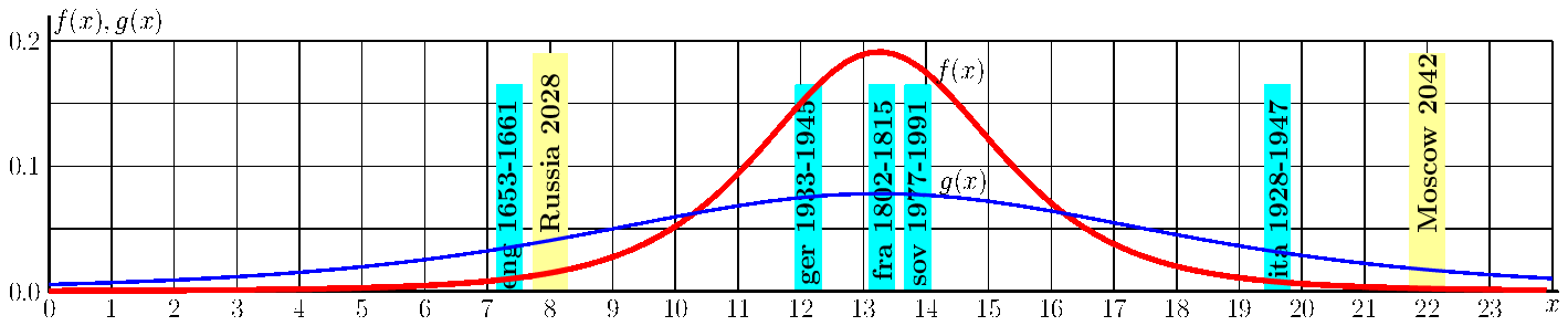
The five blue bars show the 5 observed values \(X\) of the Duration.
The two yellow bars show the values for the RF (Moscovia of century 21)
taken from the sci-fi
[14]
[15].
These "yellow" values are not taken into account at the calculus.
They shows what would the artists expect for the 6ht row of the table above - as soon as the case will be completed.
The perception of historic events by artists is not main, but still important part of History.
The blue curve refers to the similar distribution \(g\) for the next measurement \(X_{N+1}\)
under condition that the first \(N\) values are already observed;
\[
\displaystyle
g(x)= \frac{1}{c_1} \mathrm{Student}_{N-1}\!\left(
\frac{x-\tilde X}{c_1}
\right)
\]
Here parameter
\[
c_1 = s \sqrt{ 1+1/N}
\approx 4.8037 ~ \rm[years]
\]
determines the scale of the distribution.
Under condition, that the first \(N\) quantities \(X\) have given values, the probability \(p_{\rm mean}(A,B)\) that the interval \((A,B)\) includes value \(X_0\) is expressed through the likelihood density \(f\); the similar relation refers to the probability \(p_{\rm next}(A,B)\) that the interval \((A,B)\) includes value \(X_{N+1}\) that is not yet measured: \[ p_{\rm mean}(A,B)=\int_A^B f(x) \ \mathrm d x ~ ~ , ~ ~ ~ p_{\rm next}(A,B)=\int_A^B g(x) \ \mathrm d x \] For distribution densities \(f\) and \(g\), the spreads, (the «standard error»s) appear as \[ v=\sqrt{\int_{-\infty}^{\infty} f(x) \ (x\!-\!\tilde X)^2 \ \mathrm d x } ~ ~, ~ ~ w=\sqrt{\int_{-\infty}^{\infty} g(x) \ (x\!-\!\tilde X)^2 \ \mathrm d x } \] Usually it is denoted with letter \(\sigma\), but we deal with several spreads; so, we need a specific letter for each of the spreads.
Case of \(N\) observations refers to function \(\mathrm{Student}_{N-1}\). For this function, the spread is \[ \mathrm{Spread}_N=\sqrt{\int_{-\infty}^{\infty} \mathrm{Student}_{N-1}(x)\ x^2 \ \mathrm d x } = \sqrt{\frac{N-1}{N-3}} \] The mean-square deviation \(v\) of estimate \(\tilde X\) from the "true" historic constant \(X_0\) appears as follows: \[ v=c\ \sqrt{\mathrm{Dispersion}_N} = c\ \sqrt{\frac{N\!-\!1}{N\!-\!3}} = \sqrt{ \frac{1}{N(N\!-\!3)} \sum_{i=1}^N \left(X_i-\tilde X\right)^2 ~} \approx 2.7734 ~ \rm [years] \] \[ w=c_1\ \sqrt{\mathrm{Dispersion}_N} = c_1\ \sqrt{\frac{N\!-\!1}{N\!-\!3}} = \sqrt{ \frac{N+1}{N(N\!-\!3)} \sum_{i=1}^N \left(X_i\!-\!\tilde X\right)^2 ~} \approx 6.7934 ~ \rm [years] \] The formulas shows why the deal with only 3 historic cases would not be sufficient to estimate the standard error of sample mean \(\tilde X\), id est, the deviation from the "true value" \(X_0\).
In our case, roughly, the estimate \(\tilde X\) may deviate from the "true value" \(X_0\) for a quantity of order of 3 years. The next measurement \(\tilde X_{N+1}\) is expected to deviate from the estimate \(\tilde X\) for a quantity of order of 7 years.
The likelihood densities distributions \(f\) and \(g\) for these quantities are expressed through the Student Distribution with \(N\!-\!1\) degrees of freedom. Functions \(f\), \(g\) and the resulting estimates \(v\), \(w\) are main results of this model.
Note 1. The estimate \(w\) for the uncertainty of the next measurement happens to be significantly bigger, than naive estimate \[ \sqrt{c^2+s^2} \approx 4.8037 ~ ~ \rm [years] \] for the uncertainty of sum of two independent normally distributed quantities with uncertainties \(s\) and \(c\). This estimate seems to be not correct. Various naive estimates similar to that above are wifely used by the specialists. The common confusion with mistaken estimates of the uncertainties is mentioned by several authors [17] [18] [19] [20] [21].
Note 2. In this model, formally, the Duration may have negative values. This is not a big deal, while we do not declare the «Nulling» as the cause of the «Collapse». In principle, both the «Nulling» and the «Collapse» may be caused by other events and pehnomena: escalating corruption, weakness of state institutions, depletion of national resources (both natural and the «brain drain»), foreign agents of influence in the highest echelons of power, etc.; usually (but not necessary) they expolde first the Legislation of the country («Nulling»), and only then - the country («Collapse»).
In order to interpret the «Nulling» as the cause of the «Collapse», I describe another model in the section below.
Model Second is based on the following postulate:
Binary logarithms of Durations measured in years for all human civilizations, societies are distributed independently and have the same Gassian (normal) distribution with some mean value \(L_0\) and some width \(\ell_0\).
The base of the logarithm and the unit of time (e.g., years) do not serve as adjustable parameters in this model; they affect the scale of representation of data but do not affect the likelihood-based estimates or predictions.
Whitin this model, we have \(N\) measurements \(L_i=\log_2(X_i)\) and these logarithms are independent random quantities distributed with the same parameters \(L_0\) and \(\ell_0\).
From these values, I try to estimate \(L_0\), \(\ell_0\) and plot
the likelihood distribution density \(F\) for the estimate \(T=\tilde L\) and
the likelihood distribution density \(G\) for next measurement \(L_{N+1}=\log_2(X_{N+1})\) and
the likelihood distribution density \(h(x)=\frac{G(\log_2(x))}{x \ \ln(2)}\) for the next measurement \(X_{N+1}=\exp_2(L_{N+1})\).
For this model, denoting various estimates, I use capital Latin letters, to avoid confusion with analogous parameters of Model First denoted with the lowercase letters.
I calculate the sample mean value \[ T=\tilde L=\frac{1}{N} \sum_{i=1}^N L_i \approx 3.6596 \] This mean value corresponds to duration \[ \exp_2(T)≈12.636885 \approx 12.6369 ~ \rm[years] \]
This quantity appears as mean geometric value of \(N\) observed values of Duration. As expected, the mean geometric happens to slightly less than the mean arithmetic, id est, the sample mean.
Continue the similar calculations, as in Model First, I evaluate the sample variance \[ S=\sqrt{\frac{1}{N-1} \sum_{i=1}^N (L_i-T)^2\ } \approx 0.5099 \] and the scale \(C\) for the Student distribution of the sample mean \[ C=\frac{S}{\sqrt{N}}=\sqrt{\frac{1}{(N\!-\!1)N} \sum_{i=1}^N (L_i-T)^2\ } \approx 0.2280 \]
Now I express the likelihood distribution density \(F(L)\) for the mean value \(L_0\) to have value \(L\):
\[
F(L)=\frac{1}{C}\ \mathrm{Student}_{N-1}\!\left(\frac{L-T}{C}\right)
\]
This function is shown with red curve in the figure:
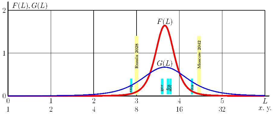
The blue bars show the 5 observed values of the logarithm, id est, \(L_i=\log_2(X_i)\).
The yellow bars show the two values from sci-fi (that are not taken into account at the computation).
The blue curve shows the likelihood density function \(G(L)\) for the logarithm \(L_{N+1}\)
of the next measurement to gets value \(L\), under condition that previous \(N\) measurements gave values \(L_i\)):
\[
G(L)=\frac{1}{C_1}\ \mathrm{Student}_{N-1}\!\left(\frac{L-T}{C_1}\right)
\]
In analogy with Model First, the parameter \(C_1\) is estimated as follows:
\[
C_1=S\ \sqrt{1+1/N} \approx 0.5585
\]
In the similar way I evaluate the spread for the sample mean and the spread \(V\) the sample mean
\[
V=\sqrt{\int_{-\infty}^{\infty} F(L) \ (L-T)^2 \ \mathrm d L\ }
=\sqrt{
\frac{N\!-\!1}{N\!-\!3}\ } \ C \approx 0.3225
\]
and the spread for the estimate \(T\!=\!\tilde L\) for the next value:
\[
W=\sqrt{\int_{-\infty}^{\infty} G(L) \ (L-T)^2 \ \mathrm d L\ }
=\sqrt{
\frac{N\!-\!1}{N\!-\!3}\ } \ C_1 \approx 0.7899
\]
As in the Model First, this spread is bigger than the naive (wrong) estimate
\[
\sqrt{C^2+S^2} \approx 0.5585
\]
Finally, I evaluate the sigma interval for the next value of \(L\):
\[
T \pm W \approx 2.8697,4.4494
\]
and for the next value \(X_{N+1}\) in this model:
\[
\exp_2(T \pm W) \approx 7.3091 , 21.8481
~ \rm [years]
\]
Functions \(F\), \(G\) and the interval \((7.3091, 21.8481)\) are the main results of the Model Second.
These are values that are supposed to be compared with the next measurement - perhaps, as soon as the row 6 in the First Table be completed.
The two models above show that the mean value of Duration is similar to its spread. This provokes the seduction to suggest even simpler model with single adjusting parameter (mean value) instead of two (mean value and the spread). Such a model is considered in this section.
Assume, that in our era, any prosper and/or powerful country has 5 relatively independent branches of power,
5 basic institurions:
1. Legislative branch (making and modifying the the Laws, parliament)
2. Executive branch (government, President, prefectures, police, army)
3. Judical branch (Courts, judges)
4. Informative branch (TV, internet, radio, newspapers)
5. Religious branch (religious communities, Churches, Synagogues, Mosques, etc.)
Assume, the usurper and his accomplices dismount the institutions mentioned, replace them with the imitations, one by one; and fall of each of them appears as the exponential decay. This leads to the model with the cascade of exponential decays.
Assume that all the decay rates per each institution mentioned are equal. (Anyway, we have no way to estimate decay rate of each institution having only 5 mrasurements.)
The assumptions above lead to the model with single parameter. The probability distribution density appears as Gamma Distribution with \(\alpha=5\) degrees of freedom. Hope, the number of degrees of freedom \(\alpha=5\) in this model will not be confused with number \(N=5\) of values of Duration, available at the moment of preparation of this article.
The resulting probability density function \[\psi(x)=\mathrm{Gamma}(\alpha, \theta, x)= \frac{1}{\Gamma(\alpha) \ \theta^\alpha} \ x^{\alpha-1} \exp(-x/\theta) \] Here, character \(\Gamma\) denotes the Gamma function; \(\Gamma(z)= (z\!+\!1)!\)
For this distribution, the mean value \[ \int_0^{\infty} \psi(x) \ x \ \mathrm dx = \theta\alpha \] As \(\alpha\) is already fixed, the native estimate for the second parameter is just \[ \theta=\tilde X/\alpha= t / 5 \approx 2.6500 ~ \rm[years] \] At least, such a choice reproduces the sample mean value.
The spread is estimated as follows: \[ \sqrt{ \int_0^{\infty} \psi(x) \ (x-t)^2 \ \mathrm dx } = \sqrt{\alpha}\theta = \frac{\tilde X}{\sqrt{\alpha}} = \frac{t}{\sqrt{\alpha}} \approx \frac{13.2498}{\sqrt{5}} \approx 5.9255 ~ \rm[years] \]
In this model, each branch of power lasts of order of 3 years before to fall allowing the next one also to fall, to collapse, to decay with the similar rate; each crime in the chain appears as a trigger of the next crime, until the collapse of the country.
Similar mechanism scaled down to only few participants makes the plot of movie «The Domino Principle 1977»
[22].
While we do not know exact mean value \(X_0\), we have to interpret function \(\psi\) as an approximation, even within this model; so \(\psi\) appears as a likelihood density distribution. This function is compared to similar functions for the other two models (Model First and Model Second) in the next section.
It may have sense to compare predictions of the 3 models above.
For this comparison, I express the likelihood density function \(h(x)\) for the next value \(X_{N+1}\) to get value \(x\) in Model Second: \[ h(x)=\frac{G\big(\log_2(x)\big)}{x \ \ln(2)} ~ \rm [years^{-1}] \] This function is shown with the black curve in the figure below:
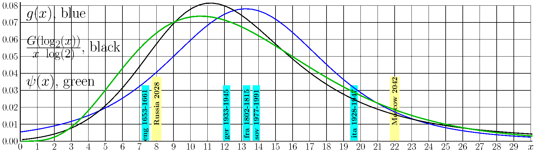
For comparison, the likelihood density \(g(x)\) for the next
value \(X_{N+1}\)
to have value \(x\) in the Model First is shown with blue line; it is the same curve as the blue curve in section about Model First; the only scale in the ordinate axis is a little bit stetted to show better curves.
The dark green curve represents likelihood density distribution for the next measurement in Model Third; it is scaled Gamma Distribution with 5 degrees of freedom; the scale is chosen to reproduce the sample mean \(\tilde X\).
The blue and yellow bars are repeated from the picture of section «Model First»;
so, I do not describe them again.
Finally, the estimates for the two models above are compared in the table below:
| Quantity | Normal distribution of durations | Normal distribution of the binary logarithms |
|---|---|---|
| Distribution | \( X \sim \mathcal{N}(X_0, \sigma_0^2) \) | \( L = \log_2 X \sim \mathcal{N}(L_0, \ell_0^2) \) |
| mean; \(N\!=\!5\) | \(t=\frac{1}{N} \sum_{n=1}^N X_n\approx13.2498\) [y.] | \(T=\frac{1}{N} \sum_{n=1}^N L_n\approx 3.6596\) \(\exp_2(T)\approx12.6369\) [y.] |
| samle spread | \(s=\sqrt{\frac{1}{N-1} \sum_{n=1}^N (X_n-t)^2}\approx 4.3851\) [y.] | \(S=\sqrt{\frac{1}{N-1} \sum_{n=1}^N (L_n-T)^2}\approx 0.5099\) |
| scale for Student | \(c=\sqrt{\frac{1}{(N-1)N} \sum_{n=1}^N (X_n\!-\!t)^2}\approx 1.9611\) [y.] | \(C=\sqrt{\frac{1}{(N-1)N} \sum_{n=1}^N (L_n\!-\!T)^2}\approx 0.2280\) |
| Density for mean | \(f(x)=\frac{1}{c} \mathrm{Student}_{N-1}\!\left( \frac{x-t}{c}\right) \ ~ \) [y.\(^{-1}\)] | \(F(L)=\frac{1}{C} \mathrm{Student}_{N-1}\!\left( \frac{L-T}{C}\right)\) |
| Spread for mean | \(v= \sqrt{ \int_{-\infty}^{\infty} f(x) ~ (x\!-\!t)^2 \ \mathrm d x \ }\) \( = \sqrt{\frac{N-1}{N-3}}\ c \approx 2.7734\ \) [y.] |
\(V= \sqrt{ \int_{-\infty}^{\infty} F(L) ~ (L\!-\!T)^2 \ \mathrm d L \ }\) \( = \sqrt{\frac{N-1}{N-3}}\ C \approx 0.3225\) |
| scale for Next | \(c_1 = s \sqrt{1+1/N}\approx 4.8037\) [y.] | \(C_1 = S \sqrt{1+1/N}\approx 0.5585\) |
| density for Next | \(g(x)=\frac{1}{c_1} \mathrm{Student}_{N-1}\!\left( \frac{x-t}{c_1}\right) \ ~ \) [y.\(^{-1}\)] | \(G(L)=\frac{1}{C_1} \mathrm{Student}_{N-1}\!\left( \frac{L-T}{C_1}\right)\) |
| Spread for Next | \(w= \sqrt{ \int_{-\infty}^{\infty} g(x) ~ (x\!-\!t)^2 \ \mathrm d x \ }\) \( = \sqrt{\frac{N-1}{N-3}}\ c_1 \approx 6.7934\ \) [y.] |
\(W= \sqrt{ \int_{-\infty}^{\infty} G(L) ~ (L\!-\!T)^2 \ \mathrm d L \ }\) \( = \sqrt{\frac{N-1}{N-3}}\ C_1 \approx 0.7899\) |
| Naive for next | \(\sqrt{s^2+c^2}\approx 4.8037 ~ \) [y.] | \(\sqrt{S^2+C^2}\approx 0.5585 \) |
| sigma interval for mean | \(t\pm v\approx 10.4764, 16.0232 ~ \) [y.] | \(T\pm V\approx 3.3371, 3.9820 ~ \) \( \exp_2( T\pm V) \approx 10.1058, 15.8020 ~ \) [y.] |
| sigma interval for next | \(t\pm w\approx 6.4564, 20.0433 ~ \) [y.] | \(T\pm W\approx 2.8697, 4.4494 ~ \) \( \exp_2( T\pm W) \approx 7.3091, 21.8481 ~ \) [y.] |
In the Gamma-based Model 3, there is no predictive likelihood function for \(X_{N+1}\) that could be an analogy of the Student distribution, as in the case of Model First and Model Second. Any such predictive density depends on prior assumptions and/or parameterization choices. For this reason, Model 3 is not included in Table 2: most of the statistics listed there - especially the likelihood density for the next measurement - lack direct analogues in the Gamma-based model, unless further assumptions are made.
In model Third, the mean for the next value is the same as Model First;
\(t\!\approx\!13.2498 \) [y].
The estimate of the spread
\(\approx\! 5.9255\) [y.] of the next value \(X_{N+1}\)
is also similar to
\(w\!\approx\! 6.7934\) [y.] in Model First.
However, in the Model Third, the spread for the next value depends on number \(\alpha\) of branches of power we have counted.
This number appears as a priori information about the Gamma Distribution used in Model Third.
In the consideration above, each of Model First and Model Second has distribution density with two adjusting parameters,
they determine the position of the maximum and the width.
Model Third, as we fix the number of degree of freedom (Five principal branches of power), has only one parameter;
the position of the maximum becomes entangled with the width. In this sense, Model Third is simpler than Model First and Model Second.
Below is an attempt to present even simpler "model".
This section provides an estimate that does not rely on any parametric model of the distribution of Duration. It gives a distribution-free forecsat for the next value of Duration.
Assume that \(D_1, \dots, D_{N+1}\) are independent and identically distributed continuous random variables.
Consider the probability that the \((N\!+\!1)\)-th observation exceeds all previous ones: \[ P\big(D_{N+1} > \max(D_1, \dots, D_N)\big). \] Since all \((N\!+\!1)!\) orderings of the sample are equally likely, and in exactly \(N!\) of them the last observation is the largest, we obtain: \[ P\big(D_{N+1} > \max(D_1, \dots, D_N)\big) = \frac{N!}{(N+1)!} = \frac{1}{N+1}. \] For \(N=5\), this gives: \[ P = \frac{1}{6} \approx 0.17 \] Therefore, with probability \(5/6 \approx 83\%\), the next observation does not exceed the maximum of the observed sample.
In the present data, the maximal observed duration is approximately 19.6 years. Thus, under the assumptions above, the next duration is expected to be below this value with probability about 83%.
This estimate is distribution-free and does not depend on the specific models considered in the previous sections. It relies only on the assumption of independent and identically distributed observations.
One can calculate with finger the number of squares of the grid lines below the hight hand side of the curves in the figure of the previous section and confirm, that the Simple Estimate shows qualitative agreement with the 3 more complicated models.
The 3.5 models above suggest that after approximately 13 years since the Federal Law breaks the principle of separation of powers («Nulling»), the republic, the empire collapses and the administrative system has to be reinstalled. All the models suggest, that Duration of any country after such a Nulling is of order of 13 years plus-minus 6 years.
Several decimal digits are kept in the estimates above in order to simplify the tracing of the computation.
Colleagues may repeat the calculus and get the same values. However, only the first two digits there have some predictive sense.
The precision of the predictions is not too good.
The estimate of the error of
the estimate of the Duration
for a next case happens to be comparable to its value.
Adding of new cases can enrich the statistics;
improving the precision of the estimate \(\tilde X\) of some "true mean value" \(X_0\)
within each of the models.
The precision of prediction of Duration for any new case is expected to remain of order of few years.
In such a way, we seem to reach the limit of the models.
The improvement of the precision of the forecast seem to require taking into account
other parameters of an empire, that pretends to be a republic but eliminates the Separation of powers.
The phenomenological modeling could be performed if more cases are added to Table 1.
The precision of prediction of Duration in the models suggested is not so high.
Several digit are kept in the estimates in order to simplify the tracing of the calculus described.
Practically, the results of all the 3 models are similar.
Since the elimination of Separation of powers, the state lasts from few years to a couple of tens of years.
The low precision is typical for primitive models.
The estimate for the Collapse of the USSR by Andrei Amalrik
[13]
also happened to be not so precise; the relative error of the prediction happens to be of order of 50%.
In 1969, Amalrik expected the USSR to collapse to year
1984 (1984-1969=15 [years]) while it collapsed, roughly, in 1991, id est, lasted 22 years (1991-1969=22 [years]) instead of 15 years expected.
Attempts of the usurpation of the superior power are observed in various epochs and in various countries. Stable democracies resist it, giving no way to apply the models above.
The attempt of American President to break the American Constitution and to serve the third Presidential term [23] Is depicted in movie «Civil War 2024» [24]. Such a destruction of the Constitution can be interpreted as elimination of Separation of powers, Nulling. Many artists consider the Nulling as dangerous. As the proof, few examples of the relevant cartoons are included below:


At the moment of preparation of this article, no document is found to confirm the successful passing of such a project through the legislative system of the USA. In sigh a way, yet, within the models considered, no certain prediction about the collapse of USA can be formulated. However, if success of the project «Trump Forever» in the USA Congress and the USA Senate, then the American case falls into the area of applicability of the models suggested and also can be used for the testing. The same may refer to any other country. There are may countries that can be qualified as authoritaric or even totalitaric. However, for them, I did not found a document that would declare siuch a totalitarism in a Federal Law. The date of publication of such a document starts the timer to count the duration. Without such a publication, the models above cannot be applied. In such a way, the range of the applicability of the models suggested happens to be very limited.

However, the models still can be applied to the 6th raw in the First Table.
The precedent cases of such a Collapse happened at the background of a big war.
There is no reason for the 6th case in the table to be an exception
[25].
The models above indicate that the treat from side of RF of century 21, see the screenshot at right,
should be considered seriously; the European countries may consider to prepare the resistance.
In particular, the analysis above may be important for the Baltic countries,
in order that the new aggression does not meet them unprepared - as it happened since 2014 with Ukraine, causing
the annexation of Crimea, the «dvizhuha» and millions victims.
If the analysis above helps to avoid the repetition of such a scenario,
then this should be the first application of the models above.
The irreversible modification of the Federal Law that esplicitly eliminates the separation of powers and allows the leader to keep the superior power is qualified as Nulling.
Duration is defined as time between the two events:
1. Nulling: The federal law of an empire eliminates the previously declared separation of powers.
2. Collapse: The empire collapses, its political and administrative system is reinstalled.
For Duration, the 6 examples are mentioned in Table 1.
At the moment of loading of the article, the last, 6th case is not yet completed,
but it can be used for the future testing the models suggested. The case is espected to be completed before 2042.
The three models are considered
with the Normal Distribution of Duration (Model First),
with the Normal Distribution of logarithm of Duration (Model Second) and
with the Gamma Distribution of Duration (Model Third).
All the three models give similar predictions for the next value of Duration; it is expected to be of order of 13 years.
The primitive estimate suggests that the next Duration will be no longer than 20 years with signoficance level 83%.
The likelihood distribution density \(f(t)\) for the mean Duration \(X_0\) to have value \(x\) and
the likelihood distribution density \(F(L)\) for the mean binary logarithm of Duration \(L_0\) to have value \(L\)
are shown in the figures for these two models.
The likelihood density for the next valuie \(X_{N+1}\) to have value \(x\)
is plotted in the last graphic for all the 3 models above.
In Model First, it is expressed with function \(g(x) ~ \rm [years^{-1}]\) through the Student Distribution.
In Model Second, it is expressed with function \(h(x)=\frac{G(\log_2(x))}{x\ \log(2)} ~ \rm [years^{-1}]\)
In Model Third, it is expressed through the Gamma Distribution
All the models suggested give similar predictions about any country
that at the level of the Federal Law abandons the principle of Separation of powers:
the administrative system of such a country is expected to last approximately 11-13 years (from 5 to 22 years) after such a Nulling.
These estimates shows also qualitative agreement with independent forecasts from the sci-fi (years 2028 and 2042).
The models and the estimates above will be verified or refuted with the last example in the First table. That case is supposed to be concluded no later than in 2042.


The analysis above is performed and uploaded with Scientific goals.
It should not be interpreted as an attempt to affect the policy of any country, nor to save the separation of powers.
If the people of some country like an «Alternative Math»[26], then, probably, their country goes to the Nulling and to the following Collapse [24] [27] [28]. In such a case, no scientific analysis can help them.
However, even in this case, Editor still keeps his right to call things with their proper names, to suggest definitions for the confusing terms, to upload the historic models and to compare their predictions to a posteriory observations (later publications).