Difference between revisions of "Fourier-2 transform"
m (Text replacement - "\$([^\$]+)\$" to "\\(\1\\)") |
|||
| (One intermediate revision by one other user not shown) | |||
| Line 1: | Line 1: | ||
'''Fourier-2 transform''' is bidimensional [[Fourier transform]] |
'''Fourier-2 transform''' is bidimensional [[Fourier transform]] |
||
| − | The transform |
+ | The transform \(g\) of a function \(f\) is defined with expression |
| − | : |
+ | : \( \displaystyle |
| − | \!\!\!\!\!\!\!\!\!\!\!\!\!\!\!\! g(x,y)= \frac{1}{2\pi} |
+ | \!\!\!\!\!\!\!\!\!\!\!\!\!\!\!\! g(x,y)= \frac{1}{2\pi} \) \(\displaystyle\iint \mathrm dp ~\mathrm dq~ \exp(-i p x - i q y ) ~ f(p,q) \) |
The Fourier transform can be used for the filtering of the function. An example of such a filtering is suggested below. |
The Fourier transform can be used for the filtering of the function. An example of such a filtering is suggested below. |
||
==Example== |
==Example== |
||
| − | [[File:Fafo2test0.png|256px|right|thumb| image of function |
+ | [[File:Fafo2test0.png|256px|right|thumb| image of function \(f\) ]] |
In this section, the example of the Fourier-2 transform of the example of the real function is considered. |
In this section, the example of the Fourier-2 transform of the example of the real function is considered. |
||
| − | For the example, the function |
+ | For the example, the function \(f\) is defined with expression |
| − | : |
+ | : \( %\displaystyle |
| − | \!\!\!\!\!\!\!\!\!\!\!\!\!\!\!\! (0) ~ ~ ~ f(x,y) = |
+ | \!\!\!\!\!\!\!\!\!\!\!\!\!\!\!\! (0) ~ ~ ~ f(x,y) =\) \(\left\{ |
\begin{array}{ll} |
\begin{array}{ll} |
||
0,&~ \text{for}~ 0.3x^2\!+\!0.2 y^2\!>\!3~\\ |
0,&~ \text{for}~ 0.3x^2\!+\!0.2 y^2\!>\!3~\\ |
||
| Line 24: | Line 24: | ||
\end{array} |
\end{array} |
||
\right. |
\right. |
||
| + | \) |
||
| − | $ |
||
| − | This function is shown in figure at right; the brightness of the rectangle at the node of the grid is proportional to value |
+ | This function is shown in figure at right; the brightness of the rectangle at the node of the grid is proportional to value \(f\) at this point. (By definition, this \(f\) has real non–negative values, either 0 or unity. The grid as \(N\!=\!64\) nodes in each direction; the step of the grid is |
| − | + | \( d = \sqrt{2 \pi/N} \approx 0.3133~\). |
|
| − | [[File:Fafo2test1.png|256px|left|thumb|image of the discrete analogy of |
+ | [[File:Fafo2test1.png|256px|left|thumb|image of the discrete analogy of \(g\) by(1)]] |
| − | The grid covers the range from |
+ | The grid covers the range from \(-\frac{N}{2}d \!\approx\! -10.0265\) to \(\frac{N-1}{2}d \!\approx |
| − | \! 9.86985~ |
+ | \! 9.86985~\). The origin of coordinates is shown with red cross. The same grid is used for all the functions evaluated below. |
| − | The modulus of the numerical evaluation of the Fourier-2 transform |
+ | The modulus of the numerical evaluation of the Fourier-2 transform \(g\) of function \(f\) is shown in the figure at left. The function approximates |
| − | : |
+ | : \( \displaystyle |
| − | \!\!\!\!\!\!\!\!\!\!\!\!\!\!\!\! (1) ~ ~ ~ g(x,y)= |
+ | \!\!\!\!\!\!\!\!\!\!\!\!\!\!\!\! (1) ~ ~ ~ g(x,y)=\) \(\frac{1}{2\pi} \) \(\displaystyle\iint \mathrm dp ~\mathrm dq~ \exp(-i p x - i q y ) f(p,q) \) |
| − | At the central spot, |
+ | At the central spot, \(g(0,0)\) is large, while at the lateral spots its values are or order of magnitude smaller; these regions are barely seen at the good resolution of the display. |
| − | [[File:Fafo2test2.png|256px|riight|thumb|image of filtered |
+ | [[File:Fafo2test2.png|256px|riight|thumb|image of filtered \(\tilde f\) by (2)]] |
| − | [[File:Fafo2test3.png|256px|riight|thumb|image of filtered |
+ | [[File:Fafo2test3.png|256px|riight|thumb|image of filtered \(\tilde f\) by (3)]] |
| − | The inverse Fourier-2 transform of |
+ | The inverse Fourier-2 transform of \(g\) coincides with \(f\), |
| − | : |
+ | : \( \displaystyle |
| − | \!\!\!\!\!\!\!\!\!\!\!\!\!\!\!\! (1.1) ~ ~ ~ f(x,y)= |
+ | \!\!\!\!\!\!\!\!\!\!\!\!\!\!\!\! (1.1) ~ ~ ~ f(x,y)=\) \(\displaystyle\frac{1}{2\pi} \) \(\displaystyle\iint \mathrm dp ~\mathrm dq ~\exp(i p x+ i q y )~ g(p,q) \) |
| − | However, another function |
+ | However, another function \(\tilde f\) appears, if the high Fourier– components are suppressed. The two examples of such a Foutier –filtering are shown in the last two figures: |
| − | : |
+ | : \( \displaystyle |
| − | \!\!\!\!\!\!\!\!\!\!\!\!\!\!\!\! (2) ~ ~ ~ \tilde f(x,y)= |
+ | \!\!\!\!\!\!\!\!\!\!\!\!\!\!\!\! (2) ~ ~ ~ \tilde f(x,y)=\) \(\displaystyle\frac{1}{2\pi} \) \(\displaystyle\iint \mathrm dp \mathrm dq ~\exp(i p x+ i q y) ~g(p,q) ~\exp(-0.04(q^2+p^2))\) |
and |
and |
||
| − | : |
+ | : \( \displaystyle |
| − | \!\!\!\!\!\!\!\!\!\!\!\!\!\!\!\! (3) ~ ~ ~ \tilde f(x,y)= |
+ | \!\!\!\!\!\!\!\!\!\!\!\!\!\!\!\! (3) ~ ~ ~ \tilde f(x,y)=\) \(\displaystyle\frac{1}{2\pi} \) \(\displaystyle\iint \mathrm dp \mathrm dq ~\exp(i p x+ i q y )~ g(p,q) ~\vartheta(20-p^2-q^2)\) |
| − | where |
+ | where \(\vartheta\) is the [[unit step function]], |
| − | : |
+ | : \( \displaystyle |
\vartheta(x)=\left\{ \begin{array}{c} 0~,~ x\le 0 \\ 1~,~ x>0\end{array} \right. |
\vartheta(x)=\left\{ \begin{array}{c} 0~,~ x\le 0 \\ 1~,~ x>0\end{array} \right. |
||
| + | \) |
||
| − | $ |
||
The examples of this section show, how the filtration in the Fourier-plane smooths the sharp image. |
The examples of this section show, how the filtration in the Fourier-plane smooths the sharp image. |
||
| Line 94: | Line 94: | ||
2D Fourier Transforms |
2D Fourier Transforms |
||
</ref>, the term "Two-Dimensional Fourier Transform" is often used in other meanings. |
</ref>, the term "Two-Dimensional Fourier Transform" is often used in other meanings. |
||
| − | In particular, the transform from |
+ | In particular, the transform from \(f\) to \(F\) with exoression |
| − | : |
+ | : \( \displaystyle F(u,v)= \int_0^\infty \mathrm d x \int_0^\infty \mathrm d y ~ ~ |
| − | f(x,y) \exp\!\big( -j 2 \pi(u x + v y) \big) |
+ | f(x,y) \exp\!\big( -j 2 \pi(u x + v y) \big)\) |
| − | where |
+ | where \(j\) has sense of \(\pm \mathrm i =\sqrt{-1}~\), is alo called "Two-Dimensional Fourier Transform". |
The same refers to the discrete analogies, which are also called "2D Fourier Transforms" |
The same refers to the discrete analogies, which are also called "2D Fourier Transforms" |
||
<ref name="jp"> |
<ref name="jp"> |
||
Latest revision as of 18:27, 30 July 2019
Fourier-2 transform is bidimensional Fourier transform
The transform \(g\) of a function \(f\) is defined with expression
- \( \displaystyle \!\!\!\!\!\!\!\!\!\!\!\!\!\!\!\! g(x,y)= \frac{1}{2\pi} \) \(\displaystyle\iint \mathrm dp ~\mathrm dq~ \exp(-i p x - i q y ) ~ f(p,q) \)
The Fourier transform can be used for the filtering of the function. An example of such a filtering is suggested below.
Example
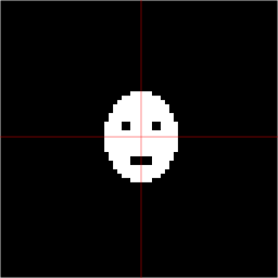
In this section, the example of the Fourier-2 transform of the example of the real function is considered.
For the example, the function \(f\) is defined with expression
- \( %\displaystyle \!\!\!\!\!\!\!\!\!\!\!\!\!\!\!\! (0) ~ ~ ~ f(x,y) =\) \(\left\{ \begin{array}{ll} 0,&~ \text{for}~ 0.3x^2\!+\!0.2 y^2\!>\!3~\\ & \mathrm{or}~ (|x|\!<\!0.8~,~ |y\!+\!1.3|<0.3) \\ & \mathrm{or}~ (|x\!-\!0.8|\!<\!0.2,~ |y\!-\!0.8|\!<\!0.2)\\ & \mathrm{or}~ (|x\!+\!0.8|\!<\!0.2,~ |y\!-\!0.8|\!<\!0.2) \\ 1 ,~ \text{over-vice} \end{array} \right. \)
This function is shown in figure at right; the brightness of the rectangle at the node of the grid is proportional to value \(f\) at this point. (By definition, this \(f\) has real non–negative values, either 0 or unity. The grid as \(N\!=\!64\) nodes in each direction; the step of the grid is \( d = \sqrt{2 \pi/N} \approx 0.3133~\).
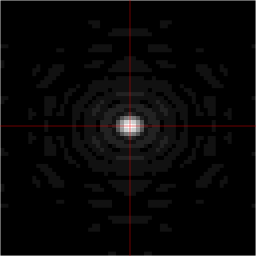
The grid covers the range from \(-\frac{N}{2}d \!\approx\! -10.0265\) to \(\frac{N-1}{2}d \!\approx \! 9.86985~\). The origin of coordinates is shown with red cross. The same grid is used for all the functions evaluated below.
The modulus of the numerical evaluation of the Fourier-2 transform \(g\) of function \(f\) is shown in the figure at left. The function approximates
- \( \displaystyle \!\!\!\!\!\!\!\!\!\!\!\!\!\!\!\! (1) ~ ~ ~ g(x,y)=\) \(\frac{1}{2\pi} \) \(\displaystyle\iint \mathrm dp ~\mathrm dq~ \exp(-i p x - i q y ) f(p,q) \)
At the central spot, \(g(0,0)\) is large, while at the lateral spots its values are or order of magnitude smaller; these regions are barely seen at the good resolution of the display.
The inverse Fourier-2 transform of \(g\) coincides with \(f\),
- \( \displaystyle \!\!\!\!\!\!\!\!\!\!\!\!\!\!\!\! (1.1) ~ ~ ~ f(x,y)=\) \(\displaystyle\frac{1}{2\pi} \) \(\displaystyle\iint \mathrm dp ~\mathrm dq ~\exp(i p x+ i q y )~ g(p,q) \)
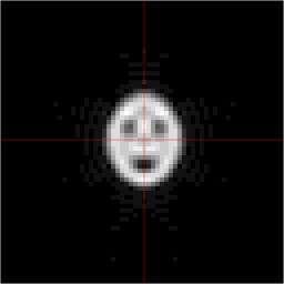
However, another function \(\tilde f\) appears, if the high Fourier– components are suppressed. The two examples of such a Foutier –filtering are shown in the last two figures:
- \( \displaystyle \!\!\!\!\!\!\!\!\!\!\!\!\!\!\!\! (2) ~ ~ ~ \tilde f(x,y)=\) \(\displaystyle\frac{1}{2\pi} \) \(\displaystyle\iint \mathrm dp \mathrm dq ~\exp(i p x+ i q y) ~g(p,q) ~\exp(-0.04(q^2+p^2))\)
and
- \( \displaystyle \!\!\!\!\!\!\!\!\!\!\!\!\!\!\!\! (3) ~ ~ ~ \tilde f(x,y)=\) \(\displaystyle\frac{1}{2\pi} \) \(\displaystyle\iint \mathrm dp \mathrm dq ~\exp(i p x+ i q y )~ g(p,q) ~\vartheta(20-p^2-q^2)\)
where \(\vartheta\) is the unit step function,
- \( \displaystyle \vartheta(x)=\left\{ \begin{array}{c} 0~,~ x\le 0 \\ 1~,~ x>0\end{array} \right. \)
The examples of this section show, how the filtration in the Fourier-plane smooths the sharp image. The colleagues are invited to download the sources of the figures (the figs are clickable, the codes are supplied) and modify the parameters of the filtering, observing the change of the filtered image.
Numerical Implementation
Many various software, including Matlab, Mathematica, Maple, IDL, have implemented the multidimensional Fourier-transform in a pretty general (and, perhaps, efficient) way.
The simple implementation can be based on the uni-dimentional routine fafo stored at fafo.cin
Here are few lines from the codes used to plot figures above.
z_type  *A; A=(z_type *)malloc((size_t)((M*N)*sizeof(z_type)));
z_type *b; b=(z_type *)malloc((size_t)((M)*sizeof(z_type)));
...
DO(m,M){ DO(n,N) b[n]=A[n*M+m]; fafo(b,N,1); DO(n,N) A[n*M+m]=b[n]; }
DO(n,N){ DO(m,M) b[m]=A[n*M+m]; fafo(b,M,1); DO(m,M) A[n*M+m]=b[m]; }
The type z_type is defined as complex(double); DO(x,y) is defined as for(x=0;x<y;x++)
Such an algorithm is not the most efficient, but it is fast, simple and easy to translate to other languages.
More examples
Example of bidimensional Fourier-transform is offered by Wolfram (Mathematica) [1].
Confusion with notations
In lectures [2][3], the term "Two-Dimensional Fourier Transform" is often used in other meanings. In particular, the transform from \(f\) to \(F\) with exoression
- \( \displaystyle F(u,v)= \int_0^\infty \mathrm d x \int_0^\infty \mathrm d y ~ ~ f(x,y) \exp\!\big( -j 2 \pi(u x + v y) \big)\)
where \(j\) has sense of \(\pm \mathrm i =\sqrt{-1}~\), is alo called "Two-Dimensional Fourier Transform". The same refers to the discrete analogies, which are also called "2D Fourier Transforms" [4].
Wikiedia [5] offers descriptions of various objects called "Fourier transform".
Often both, the integral operator and the result of its application to some function are called "Fourier transform".
In general, the Fourier transforms of the some function, defined in different publications, do not coincide. In particular, this apply to the bidimensional Fourier transform. Therefore, at the use, the explicit definition should be specified.
References
- ↑ http://demonstrations.wolfram.com/2DFourierTransforms/
- ↑ http://fourier.eng.hmc.edu/e101/lectures/Image_Processing/node6.html Two-Dimensional Fourier Transform
- ↑ http://www.cs.toronto.edu/~jepson/csc320/notes/linearFilters2.pdf 2D Fourier Transforms
- ↑ http://www.mathworks.co.jp/help/toolbox/images/f21-17064.html Image Processing Toolbox. Definition of Fourier Transform.
- ↑ http://en.wikipedia.org/wiki/Fourier_transform


