Search results
Create the page "Approximation" on this wiki! See also the search results found.
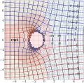
File:TaniaBigMap.png In the shaded range, the precision of the approximation is smaller than 3; the precision is defined with<br> - \lg\big( \frac{ |\mathrm{Tania}(z)-\mathrm{approximation}(z)|}(851 × 841 (654 KB)) - 08:53, 1 December 2018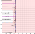
File:TaniaNegMapT.png The truncation of the series gives the approximation shown in the figure.(1,773 × 1,752 (306 KB)) - 09:39, 21 June 2013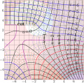
File:TaniaSinguMapT.png [[Complex map]] of the approximation of the [[Tania function]] with the truncated series of the expansion at the The shaded region indicates the range, where the precision of such an approximation of the [[Tania function]] is worse than 3.(851 × 841 (615 KB)) - 08:53, 1 December 2018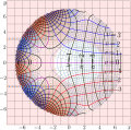
File:TaniaTaylor0T.png The range where the Taylor approximation returns less than 3 signifivant figures is shaded.(851 × 841 (650 KB)) - 09:39, 21 June 2013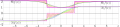
File:TetSheldonImaT.png ==Approximation==(4,359 × 980 (598 KB)) - 09:40, 21 June 2013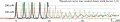
File:TodaShow.png ...znetsov, J.-F.Bisson, J.Li, K.Ueda. Self-pulsing laser as oscillator Toda: approximation of the solution through elementary functions -- J. Phys. A: 40, 2107-2124 ((1,707 × 317 (155 KB)) - 09:39, 21 June 2013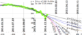
File:2014.12.26rubleDollar.png The last two columns of the table above characterise the precision of each approximation: [[Category:Approximation of rubble]](1,502 × 651 (246 KB)) - 08:26, 1 December 2018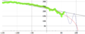
File:2014.12.29fitA300.png The red monotonous line shows the approximation the blue oscillating curve shows the approximation(1,500 × 603 (100 KB)) - 08:26, 1 December 2018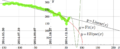
File:2014.12.29rubleDollar.png The straight black line represents the linear approximation of the data, The red monotonous line represents the approximation with ellipse,(1,502 × 610 (142 KB)) - 08:26, 1 December 2018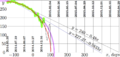
File:2014.12.31rudo.png The thick ping arc covers the approximation Primary, this approximation had been used 29 November 2014 as(1,452 × 684 (190 KB)) - 08:26, 1 December 2018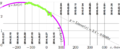
File:2014arc.png the lineal approximation of the data available 2014.10.27 (thin black straight line), and the approximation Arc, made 2014.11.29 (thick ping arc):(1,726 × 709 (155 KB)) - 08:26, 1 December 2018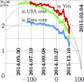
File:2014ruble15t.png ...of the project, the value of rouble becomes imaginary. According to these approximation, this may happen around 2015.02.04. [[Category:Approximation]](693 × 680 (110 KB)) - 08:26, 1 December 2018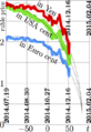
File:2014ruble17t.png [[Category:Approximation]](456 × 664 (98 KB)) - 08:26, 1 December 2018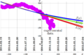
File:2014rubleDollar2param.png [[Category:Linear approximation]](1,527 × 1,004 (232 KB)) - 08:26, 1 December 2018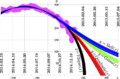
File:2014rubleDollar3param.png ...aced. The thickness of the resulting line qualifies the instability of the approximation. [[Category:Approximation]](1,273 × 837 (294 KB)) - 08:26, 1 December 2018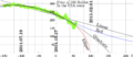
File:2014specula.png ==Linear approximation== The black straight line shows the linear approximation,(1,502 × 651 (177 KB)) - 08:26, 1 December 2018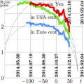
File:2014рубле16t.png [[Category:Approximation]](680 × 680 (112 KB)) - 08:26, 1 December 2018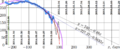
File:2015.01.01rudo.png ...ordinate is marked with green vertical line. In order to show the limit of approximation, some more data are plotted also at the left hand side of this vertical lin(1,660 × 684 (215 KB)) - 08:26, 1 December 2018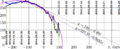
File:2015.01.03rudo.png The upper linear approximation is from 2014.10.31, shown in also figure http://mizugadro.mydns.jp/t/index. The pink arc follows the approximation(1,660 × 684 (212 KB)) - 08:26, 1 December 2018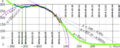
File:2015.01.05rudo.png The upper linear approximation $y=240-0.48x$ had been suggested 2014.10.31; it is shown also in figure htt This linear approximation is called also "program 500 days" (Программа 500 дней)(1,867 × 747 (271 KB)) - 08:26, 1 December 2018


