File:AcosmapT200.png

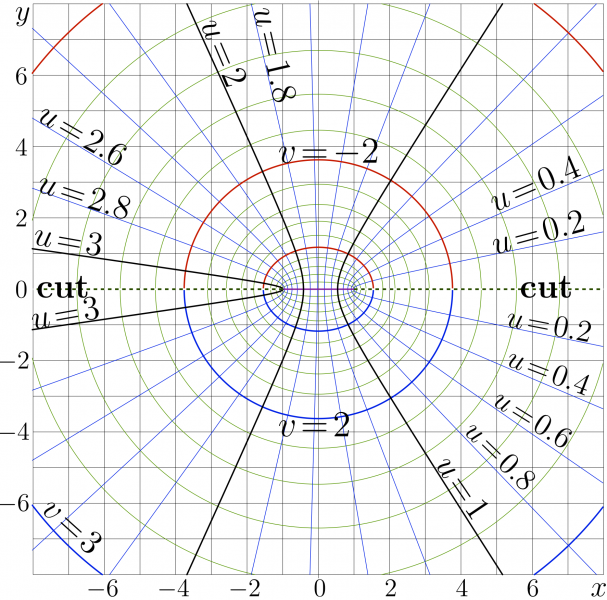
Complex map of function ArcCos.

$f=\arccos(x +\mathrm i y)$ is shown in the $x$, $y$ plane with levels $u=\Re(f)=\mathrm{const}$ and levels $v=\Im(f)=\mathrm{const}$

Thick lines correspond to the integer values.

C++ generator of curves

Files ado.cin and conto.cin should be loaded to the working directory for compilation of the C++ code below:

#include <math.h> 
#include <stdio.h>
#include <stdlib.h>
#define DB double
#define DO(x,y) for(x=0;x<y;x++)
using namespace std;
#include <complex> 
typedef complex<double> z_type;
#define Re(x) x.real() 
#define Im(x) x.imag()
#define I z_type(0.,1.)
#include "conto.cin"

 z_type acos(z_type z){
 if(Im(z)<0){if(Re(z)>=0){return I*log( z + sqrt(z*z-1.) );}
                    else{return I*log( z - sqrt(z*z-1.) );}}
            if(Re(z)>=0){return  -I*log( z + sqrt(z*z-1.) );}
                   else {return  -I*log( z - sqrt(z*z-1.) );} }

main(){ int j,k,m,n; DB x,y, p,q, t; z_type z,c,d;
int M=400,M1=M+1;
int N=401,N1=N+1;
DB X[M1],Y[N1], g[M1*N1],f[M1*N1], w[M1*N1]; // w is working array.
char v[M1*N1]; // v is working array
FILE *o;o=fopen("acosmap.eps","w");ado(o,162,162);
fprintf(o,"81 81 translate\n 10 10 scale\n");
DO(m,M1) X[m]=-8.+.04*(m-.5);
DO(n,200)Y[n]=-8.+.04*n;
      Y[200]=-.015;
      Y[201]= .015;
for(n=202;n<N1;n++) Y[n]=-8.+.04*(n-1.);
for(m=-8;m<9;m++){if(m==0){M(m,-8.5)L(m,8.5)} else{M(m,-8)L(m,8)}}
for(n=-8;n<9;n++){     M(  -8,n)L(8,n)}
fprintf(o,".01 W 0 0 0 RGB S\n");
DO(m,M1)DO(n,N1){g[m*N1+n]=9999; f[m*N1+n]=9999;}
DO(m,M1){x=X[m]; //printf("%5.2f\n",x);
DO(n,N1){y=Y[n]; z=z_type(x,y);
      c=acos(z);
      p=Re(c);q=Im(c);
      if(p>-99. && p<99. &&
         q>-99. && q<99 //&& fabs(q)> 1.e-19
      )
      {g[m*N1+n]=p;f[m*N1+n]=q;}
                      }}
fprintf(o,"1 setlinejoin 1 setlinecap\n"); p=1.8;q=.7;
for(m=-11;m<11;m++)for(n=2;n<10;n+=2)conto(o,f,w,v,X,Y,M,N,(m+.1*n),-q, q); fprintf(o,".016 W 0 .6 0 RGB S\n");
for(m=0;m<10;m++) for(n=2;n<10;n+=2)conto(o,g,w,v,X,Y,M,N,-(m+.1*n),-q, q); fprintf(o,".016 W .9 0 0 RGB S\n");
for(m=0;m<10;m++) for(n=2;n<10;n+=2)conto(o,g,w,v,X,Y,M,N, (m+.1*n),-q, q); fprintf(o,".016 W 0 0 .9 RGB S\n");
for(m=1;m<11;m++)  conto(o,f,w,v,X,Y,M,N, (0.-m),-p,p); fprintf(o,".04 W .9 0 0 RGB S\n");
for(m=1;m<11;m++)  conto(o,f,w,v,X,Y,M,N, (0.+m),-p,p); fprintf(o,".04 W 0 0 .9 RGB S\n");
                 conto(o,f,w,v,X,Y,M,N, (0.  ),-p,p); fprintf(o,".04 W .6 0 .6 RGB S\n");
for(m=-9;m<10;m++) conto(o,g,w,v,X,Y,M,N, (0.+m),-p,p); fprintf(o,".04 W 0 0 0 RGB S\n");
fprintf(o,"0 setlinecap\n");
M(-1,0)L(-8,0) M(1,0)L(8,0)
fprintf(o,"0.05 W 1 1 1 RGB S\n");
DO(m,35) {x=-1.-.2*m; M(x,0) L(x-.1,0)}
DO(m,35) {x= 1.+.2*m; M(x,0) L(x+.1,0)}
fprintf(o,".05 W 0 .3 0 RGB S\n");
fprintf(o,"showpage\n%c%cTrailer",'%','%'); fclose(o);
      system("epstopdf acosmap.eps");
      system(    "open acosmap.pdf");
      getchar(); system("killall Preview");//for mac
}

Latex generator of labels

For compilation of the Latex code below, file acosmap.pdf should be generated with the code from the previous section.

% Copyleft 2011 by Dmitrii Kouznetsov \documentclass[12pt]{article} %<br> \usepackage{geometry} %<br> \usepackage{graphicx} %<br> \usepackage{rotating} %<br> \paperwidth 854pt %<br> \paperheight 844pt %<br> \topmargin -96pt %<br> \oddsidemargin -98pt %<br> \textwidth 1100pt %<br> \textheight 1100pt %<br> \pagestyle {empty} %<br> \newcommand \sx {\scalebox} %<br> \newcommand \rot {\begin{rotate}} %<br> \newcommand \ero {\end{rotate}} %<br> \newcommand \ing {\includegraphics} %<br> \begin{document} %<br> \sx{5}{ \begin{picture}(164,165) %<br> \put(6,5){\ing{acosmap}} %<br> \put(2,162){\sx{.7}{$y$}} %<br> \put(2,144){\sx{.6}{$6$}} %<br> \put(2,124){\sx{.6}{$4$}} %<br> \put(2,104){\sx{.6}{$2$}} %<br> \put(4,134){ \sx{.8}{\rot{-30}$u\!=\!2.6$\ero}} %<br> \put(4,114){ \sx{.8}{\rot{-18}$u\!=\!2.8$\ero}} %<br> \put(3,99){ \sx{.8}{\rot{-10}$u\!=\!3$\ero}} %<br> \put(2, 84){\sx{.6}{$0$}} %<br> \put(8, 84){\sx{.8}{\bf cut}} %<br> \put(7,75){\sx{.8}{\rot{10}$u\!=\!3$\ero}} %<br> \put(-3,64){\sx{.6}{$-2$}} %<br> \put(-3,44){\sx{.6}{$-4$}} %<br> \put(-3,24){\sx{.6}{$-6$}} %<br> \put( 22,0){\sx{.6}{$-6$}} %<br> \put( 42,0){\sx{.6}{$-4$}} %<br> \put( 62,0){\sx{.6}{$-2$}} %<br> \put( 86,0){\sx{.6}{$0$}} %<br> \put(106,0){\sx{.6}{$2$}} %<br> \put(126,0){\sx{.6}{$4$}} %<br> \put(146,0){\sx{.6}{$6$}} %<br> \put(164,0){\sx{.7}{$x$}} %<br> \put( 54, 161){\rot{-67}\sx{.82}{$u\!=\!2$}\ero}%<br> \put( 69, 165){\rot{-77}\sx{.82}{$u\!=\!1.8$}\ero}%<br> \put( 76, 122){\rot{.1}\sx{.86}{$v\!=\!-2$}\ero}%<br> \put( 76, 45){\rot{-.1}\sx{.86}{$v\!=\!2$}\ero}%<br> \put( 9, 24){\rot{-42}\sx{.8}{$v\!=\!3$}\ero}%<br> \put(137, 108){\rot{23}\sx{.8}{$u\!=\!0.4$}\ero}%<br> \put(137, 96){\rot{15}\sx{.8}{$u\!=\!0.2$}\ero}%<br> \put(144, 84){\rot{0}\sx{.8}{\bf cut}\ero}%<br> \put(140, 76){\rot{-11}\sx{.72}{$u\!=\!0.2$}\ero}%<br> \put(140, 65){\rot{-21}\sx{.72}{$u\!=\!0.4$}\ero}%<br> \put(136, 54){\rot{-32}\sx{.72}{$u\!=\!0.6$}\ero}%<br> \put(128, 46){\rot{-44}\sx{.72}{$u\!=\!0.8$}\ero}%<br> \put(120, 37){\rot{-56}\sx{.8}{$u\!=\!1$}\ero}%<br> \end{picture} %<br> } %<br> \end{document}

Keywords

ArcCos, Complex map