Difference between revisions of "File:FactoriAsymptoAgreeT.png"
({{oq|FactoriAsymptoAgreeT.png|Original file (800 × 667 pixels, file size: 50 KB, MIME type: image/png)|400}} Map of agreement \[ a(z) = - \lg \left(\frac {|z!-A(z)|} {|z!|+|A(z)|} \right) \] of the asymptotic \[ A(z)= \sqrt{2\pi z}\ \exp\left(\log\left(\frac{z}{\mathrm e} \right) z + \frac{1}{12 z}\left(1+ \frac{1}{z^2}\left(\frac{-1}{30}+ \frac{1}{z^2}\left(\frac{1}{105}+ \frac{1}{z^2}\left(\frac{-1}{140}+ \frac{1}{z^2}\left(\frac{1}{99}+ \frac{1}{z^2}\left(\frac{-1}{42} \right) \rig...) |
(T uploaded a new version of File:FactoriAsymptoAgreeT.png) |
||
| (2 intermediate revisions by the same user not shown) | |||
| Line 1: | Line 1: | ||
| ⚫ | |||
| − | == Summary == |
||
| ⚫ | |||
Map of [[agreement]] |
Map of [[agreement]] |
||
| Line 28: | Line 27: | ||
with function [[Factorial]] \( z \mapsto z!\). |
with function [[Factorial]] \( z \mapsto z!\). |
||
| + | In the agreement \(A\), the [[Stirling series]] <ref> |
||
| ⚫ | |||
| + | https://mathworld.wolfram.com/StirlingsSeries.html |
||
| + | The asymptotic series for the gamma function .. |
||
| + | The series for z! is obtained by adding an additional factor of z, .. |
||
| + | </ref> is incorporated into the exponent rather than as a multiplicative polynomial. |
||
| + | However, for this example, the truncated series is used; so, here, the [[asymptotic]] \(A\) |
||
| + | is just [[Elementary function]]. |
||
| + | |||
| ⚫ | |||
| + | https://math.stackexchange.com/questions/1711804/why-use-the-logarithm-of-the-relative-error |
||
| + | Why use the logarithm of the relative error? (y.2015) .. We computed the numerical solution, plotted against the given closed form solution, and and then were told to "calculate the logarithm of the maximum relative error" .. |
||
| + | What's the idea behind taking to logarithm of this error? .. |
||
| + | </ref><ref> |
||
| + | https://www.sciencedirect.com/topics/computer-science/relative-error |
||
| + | [[Relative Error]] refers to a way of measuring the difference between an estimated or approximated value and the actual value, expressed as a ratio of the absolute difference to the actual value. .. |
||
| + | </ref>. |
||
Levels |
Levels |
||
| Line 35: | Line 49: | ||
\(a\!=\!6\), |
\(a\!=\!6\), |
||
\(a\!=\!9\), |
\(a\!=\!9\), |
||
| − | \(a\!=\!12\) are |
+ | \(a\!=\!12\) are shown as thick colored curves. |
The pink shade is an attempt to draw level |
The pink shade is an attempt to draw level |
||
\(a\!=\!15\). |
\(a\!=\!15\). |
||
| − | Apparently, the rounding errors of the complex double variables do not allow to draw the smooth contour - |
+ | Apparently, the rounding errors of the complex double variables («[[double precision]]») do not allow to draw the smooth contour - |
at least with the current implementation [[fac.cin]] of the [[Factorial]] function. |
at least with the current implementation [[fac.cin]] of the [[Factorial]] function. |
||
| − | ( |
+ | (If someone can do it better, go ahead!) |
The picture is prepared as an example for articles |
The picture is prepared as an example for articles |
||
| Line 48: | Line 62: | ||
«[[Sectorial asymptotic]]». |
«[[Sectorial asymptotic]]». |
||
| − | Also, the map serves as test for |
+ | Also, the map serves as test for routine [[Conrec6.cin]]; |
| − | the code below can be used as an example of the driver routine (program that calls the routine |
+ | the code below can be used as an example of the driver routine (program that calls the routine). |
==Interpretation== |
==Interpretation== |
||
| − | The map suggests that the asymptotic \(A(z)\) above |
+ | The map suggests that the asymptotic \(A(z)\) above |
| + | <!-- |
||
| + | returns at least 14 significant figures of |
||
| + | !--> |
||
| + | provides of order of 14 significant figures of |
||
[[Factorial]]\((z)\) in the range |
[[Factorial]]\((z)\) in the range |
||
\[ d = (\ \Re(z) \!\ge\! -6 , \ |z|\!>\!8\ )\ \lor \ (\Re(z)\!<\!-6 , \ |\Im(z)|\!>\!5 \ ) |
\[ d = (\ \Re(z) \!\ge\! -6 , \ |z|\!>\!8\ )\ \lor \ (\Re(z)\!<\!-6 , \ |\Im(z)|\!>\!5 \ ) |
||
| Line 67: | Line 85: | ||
At large \(|z|\), |
At large \(|z|\), |
||
| − | the residual \(r(z)=\)[[Factorial]]\((z) |
+ | the residual \(\ r(z)\!=\)[[Factorial]]\((z)\!-\!A(z) \ \) |
| + | remains asymptotically negligible compared to [[Factorial]]\((z)\) |
||
| − | in the whole complex \(z\) plane except arbitrary narrow sector the includes the negative part of the real axis: |
||
| + | in the whole complex \(z\) plane |
||
| + | except an arbitrarily narrow sector containing the negative real axis: |
||
\[ |
\[ |
||
\lim_{|z|\to \infty, \ z \in D} \frac{r(z)}{z!} = 0 |
\lim_{|z|\to \infty, \ z \in D} \frac{r(z)}{z!} = 0 |
||
| + | \] |
||
| + | Here, the limit is not uniform as \(\alpha\to\pi\) . |
||
| + | The mathematically precise version of the formula above can be written as follows: |
||
| + | \[ |
||
| + | \forall \alpha<\pi:\quad |
||
| + | \lim_{|z|\to\infty,\ |\arg z|\le \alpha} |
||
| + | \frac{r(z)}{z!}=0 |
||
\] |
\] |
||
| Line 157: | Line 184: | ||
system( "open FactoriAsymptoAgree.pdf"); //for mac |
system( "open FactoriAsymptoAgree.pdf"); //for mac |
||
} |
} |
||
| + | |||
</pre> |
</pre> |
||
| + | |||
==Latex== |
==Latex== |
||
%I have no idea why I have to declare paper <br> |
%I have no idea why I have to declare paper <br> |
||
| Line 215: | Line 244: | ||
\end{document} |
\end{document} |
||
</pre> |
</pre> |
||
| − | == |
+ | ==ChatGPT== |
| + | 1. [[ChatGPT]] helps to improve the description of this picture. |
||
| ⚫ | |||
| + | |||
| ⚫ | |||
This routine is tailored in collaboration with [[ChatGPT]].<br> |
This routine is tailored in collaboration with [[ChatGPT]].<br> |
||
Please attribute the source at the reuse:<br> |
Please attribute the source at the reuse:<br> |
||
the attribution helps to trace [[bug]](s) if any. |
the attribution helps to trace [[bug]](s) if any. |
||
| + | ==Notes by [[ChatGPT]]== |
||
| + | Some notes by [[ChatGPT]] are not included in the description above: |
||
| + | The pink noise at \(a\approx 15\) is **exactly what one expects** from [[double precision]] near exponential cancellation. |
||
| − | The picture generated with the C++ and the Latex above is converted to PNG with command |
||
| + | When \(|z!|\gg|A(z)-z!|\), the agreement \(a(z)\) approximately equals the number of correct decimal digits in the relative sense. |
||
| − | convert FactoriAsymptoAgreeT.pdf png8:FactoriAsymptoAgreeT.png |
||
| + | |||
| + | The degradation near the negative real axis reflects the Stokes phenomenon associated with the logarithmic [[branch cut]]. |
||
==References== |
==References== |
||
| Line 238: | Line 273: | ||
«[[Asymptotic]]», |
«[[Asymptotic]]», |
||
«[[ChatGPT]]», |
«[[ChatGPT]]», |
||
| − | «[[ |
+ | «[[Conrec6]]», |
| − | «[[ |
+ | «[[Elementary function]]», |
| − | «[[fac.cin]]» |
||
«[[Factorial]]», |
«[[Factorial]]», |
||
«[[Map]]», |
«[[Map]]», |
||
| Line 249: | Line 283: | ||
[[Category:Agreement]] |
[[Category:Agreement]] |
||
[[Category:Asymptotic]] |
[[Category:Asymptotic]] |
||
| − | [[Category:C++]] |
||
[[Category:ChatGPT]] |
[[Category:ChatGPT]] |
||
[[Category:Factorial]] |
[[Category:Factorial]] |
||
| − | [[Category:Latex]] |
||
[[Category:Map]] |
[[Category:Map]] |
||
[[Category:Restricted asymptotic]] |
[[Category:Restricted asymptotic]] |
||
Latest revision as of 19:48, 19 January 2026
Map of agreement \[ a(z) = - \lg \left(\frac {|z!-A(z)|} {|z!|+|A(z)|} \right) \] of the asymptotic \[ A(z)= \sqrt{2\pi z}\ \exp\left(\log\left(\frac{z}{\mathrm e} \right) z + \frac{1}{12 z}\left(1+ \frac{1}{z^2}\left(\frac{-1}{30}+ \frac{1}{z^2}\left(\frac{1}{105}+ \frac{1}{z^2}\left(\frac{-1}{140}+ \frac{1}{z^2}\left(\frac{1}{99}+ \frac{1}{z^2}\left(\frac{-1}{42} \right) \right) \right) \right) \right) \right) \right) \] with function Factorial \( z \mapsto z!\).
In the agreement \(A\), the Stirling series [1] is incorporated into the exponent rather than as a multiplicative polynomial. However, for this example, the truncated series is used; so, here, the asymptotic \(A\) is just Elementary function.
The agreement \(a=a(x\!+\!\mathrm i y)\) is shown with levels \(a=\mathrm{const}\) in the \(x,y\) plane. This agreement can be qualified as a logarithmic relative error measure [2][3].
Levels \(a\!=\!1\), \(a\!=\!3\), \(a\!=\!6\), \(a\!=\!9\), \(a\!=\!12\) are shown as thick colored curves.
The pink shade is an attempt to draw level \(a\!=\!15\). Apparently, the rounding errors of the complex double variables («double precision») do not allow to draw the smooth contour - at least with the current implementation fac.cin of the Factorial function. (If someone can do it better, go ahead!)
The picture is prepared as an example for articles «Asymptotic», «Restricted asymptotic», «Sectorial asymptotic».
Also, the map serves as test for routine Conrec6.cin; the code below can be used as an example of the driver routine (program that calls the routine).
Interpretation
The map suggests that the asymptotic \(A(z)\) above provides of order of 14 significant figures of Factorial\((z)\) in the range \[ d = (\ \Re(z) \!\ge\! -6 , \ |z|\!>\!8\ )\ \lor \ (\Re(z)\!<\!-6 , \ |\Im(z)|\!>\!5 \ ) \]
Function \(A\) is interpreted as Restricted asymptotic:
It is the Sectorial asymptotic of Factorial at large values of its argument for sector \[ D= \{ z\in \mathbf C \ : |\arg(z)|< \alpha \} \] where \(\alpha\) is any positive real number such that \( \alpha < \pi \).
At large \(|z|\), the residual \(\ r(z)\!=\)Factorial\((z)\!-\!A(z) \ \) remains asymptotically negligible compared to Factorial\((z)\) in the whole complex \(z\) plane except an arbitrarily narrow sector containing the negative real axis: \[ \lim_{|z|\to \infty, \ z \in D} \frac{r(z)}{z!} = 0 \] Here, the limit is not uniform as \(\alpha\to\pi\) . The mathematically precise version of the formula above can be written as follows: \[ \forall \alpha<\pi:\quad \lim_{|z|\to\infty,\ |\arg z|\le \alpha} \frac{r(z)}{z!}=0 \]
C++
/* Routines
«ado.cin»,
«Conrec6.cin»,
«fac.cin»
should be loaded for the compilation of the code below.
Options « -std=c++11 -O2 » are strongly recommended. */
// c++ -std=c++11 FactoriAsymptoAgree.cc -O2 -o FactoriAsymptoAgree
#include <math.h>
#include <stdio.h>
#include <stdlib.h>
#define DB double
#define DO(x,y) for(x=0;x<y;x++)
using namespace std;
#include <complex>
typedef complex<double> z_type;
#define Re(x) x.real()
#define Im(x) x.imag()
#define I z_type(0.,1.)
#include"ado.cin"
#define M(x,y) fprintf(o,"%6.4f %6.4f M\n",1.*(x),1.*(y));
#define L(x,y) fprintf(o,"%6.4f %6.4f L\n",1.*(x),1.*(y));
#include "Conrec6.cin"
#include "fac.cin"

z_type facas(z_type z){ z_type c=1./z; z_type d=c*c;
return sqrt(M_PI*2.*z)*exp(log(z/M_E)*z+(1./12.)*c*(
1.+d*(-1./30.+d*(1./105.+d*(-1./140.+d*(1./99.+d*(-1./42.)))))
));
//(1.+c*(1./12.+c*(1./288.+c*(-139./51840.))));
}

int main(){ int j,k,m,n; DB x,y, p,q, t; z_type z,c,d;
int M=251,M1=M+1;
int N=201,N1=N+1;
DB X[M1],Y[N1], g[M1*N1];
//,f[M1*N1];
FILE *o;o=fopen("FactoriAsymptoAgree.eps","w");ado(o,252,202);
fprintf(o,"151 101 translate\n 10 10 scale\n");

DO(m,M1) X[m]=-15+.1*(m-.5);
DO(n,N1) Y[n]=-10+.1*(n-.5);

DO(m,M1)DO(n,N1){g[m+M1*n]=9999;}
DO(m,M1){x=X[m]; //printf("%5.2f\n",x);
DO(n,N1){y=Y[n]; z=z_type(x,y);
// c=Filog(z);
//c=z*z*sin(1./z);
c=fac(z);
d=facas(z);
p= - log( abs(c-d) / (abs(c)+abs(d)) )/log(10.);
//p=Re(c);q=Im(c);
g[m+M1*n]=p;
       }}
fprintf(o,"1 setlinejoin 1 setlinecap\n"); p=5.;q=1;
p=15.;
Conrec6(o,g,X,Y,M1,N1, 1. ,p); fprintf(o,".12 W 1 0 0 RGB S\n");
Conrec6(o,g,X,Y,M1,N1, 2. ,p); fprintf(o,".04 W 0 0 0 RGB S\n");
Conrec6(o,g,X,Y,M1,N1, 3. ,p); fprintf(o,".12 W .6 .4 0 RGB S\n");
Conrec6(o,g,X,Y,M1,N1, 4. ,p); fprintf(o,".06 W 0 0 0 RGB S\n");
Conrec6(o,g,X,Y,M1,N1, 5. ,p); fprintf(o,".06 W 0 0 0 RGB S\n");
Conrec6(o,g,X,Y,M1,N1, 6. ,p); fprintf(o,".12 W 0 .8 0 RGB S\n");
Conrec6(o,g,X,Y,M1,N1, 7. ,p); fprintf(o,".06 W 0 0 0 RGB S\n");
Conrec6(o,g,X,Y,M1,N1, 8. ,p); fprintf(o,".06 W 0 0 0 RGB S\n");
Conrec6(o,g,X,Y,M1,N1, 9. ,p); fprintf(o,".12 W 0 .5 .6 RGB S\n");
Conrec6(o,g,X,Y,M1,N1, 10. ,p); fprintf(o,".06 W 0 0 0 RGB S\n");
Conrec6(o,g,X,Y,M1,N1, 11. ,p); fprintf(o,".06 W 0 0 0 RGB S\n");
Conrec6(o,g,X,Y,M1,N1, 12. ,p); fprintf(o,".12 W 0 0 1 RGB S\n");
Conrec6(o,g,X,Y,M1,N1, 13. ,p); fprintf(o,".06 W 0 0 0 RGB S\n");
Conrec6(o,g,X,Y,M1,N1, 14. ,p); fprintf(o,".06 W 0 0 0 RGB S\n");
Conrec6(o,g,X,Y,M1,N1, 15. ,p); fprintf(o,".07 W 1 .5 1 RGB S\n");

for(m=-10;m<11;m++){if(m!=0){M(m,-10)L(m,10)}}
for(n=-10;n<11;n++){M(-10,n)L(10,n)}
fprintf(o,"2 setlinecap .02 W 0 0 0 RGB S\n");
fprintf(o,"2 setlinecap .02 W 0 0 0 RGB S\n");
M(0,-10)L(0,11)
fprintf(o,"2 setlinecap .03 W 0 0 0 RGB S\n");

fprintf(o,"showpage\n%c%cTrailer",'%','%'); fclose(o);
     system("epstopdf FactoriAsymptoAgree.eps");
     system(    "open FactoriAsymptoAgree.pdf"); //for mac
}
Latex
%I have no idea why I have to declare paper
%sizes 803x669 in order to get picture of
%sizes 800x667
\documentclass[12pt]{article}
\usepackage{geometry}
\paperwidth 803pt
\paperheight 669pt
\textwidth 800pt
\textheight 700pt
\topmargin -106pt
\oddsidemargin -116pt
\usepackage{graphicx}
\usepackage{rotating}
\newcommand \rot {\begin{rotate}}
\newcommand \ero {\end{rotate}}
\newcommand \rme {\mathrm{e}}
\newcommand \sx {\scalebox}
\begin{document}
\sx{3.15}{\begin{picture}(230,211)
\normalsize
%\put(40,0){\ing{oblakoV}}
%\put(10,10){\includegraphics{Z2sin1zMap}}
\put(10,8){\includegraphics{FactoriAsymptoAgree}}
\put(53,204){\sx{1.2}{\(y\)}}
\put(53,185){\sx{1.1}{\(8\)}}
\put(53,165){\sx{1.1}{\(6\)}}
\put(53,145){\sx{1.1}{\(4\)}}
\put(53,125){\sx{1.1}{\(2\)}}
\put(53,105){\sx{1.1}{\(0\)}}
\put(44,85){\sx{1.1}{\(-2\)}}
\put(44,65){\sx{1.1}{\(-4\)}}
\put(44,45){\sx{1.1}{\(-6\)}}
\put(44,25){\sx{1.1}{\(-8\)}}
\put(45, 0){\sx{.9}{\(-10\)}}
\put(73, 0){\sx{.9}{\(-8\)}}
\put(93, 0){\sx{.9}{\(-6\)}}
\put(113, 0){\sx{.9}{\(-4\)}}
\put(133, 0){\sx{.9}{\(-2\)}}
\put(159, 0){\sx{.9}{\(0\)}}
\put(179, 0){\sx{.9}{\(2\)}}
\put(199, 0){\sx{.9}{\(4\)}}
\put(219, 0){\sx{.9}{\(6\)}}
\put(239, 0){\sx{.9}{\(8\)}}
\put(256, 0){\sx{1.1}{\(x\)}}
%\put(8,194){\sx{1.4}{\rot{0}\(a\!\approx\!15\) \ero} }
%\put(132,196){\sx{1.6}{\rot{0}\(a\!\approx\!15\) \ero} }
%\put(132,176){\sx{1.6}{\rot{0}\(a\!=\!14\) \ero} }
%\put(132,156){\sx{1.6}{\rot{0}\(a\!=\!12\) \ero} }

\put(185,52){\sx{1.6}{\rot{42}\(a\!=\!12\) \ero} }
\put(203,37){\sx{1.6}{\rot{40}\(a\!=\!14\) \ero} }
\put(212,19){\sx{1.6}{\rot{37}\(a\!\approx\!15\) \ero} }
\end{picture}}
\end{document}
ChatGPT
1. ChatGPT helps to improve the description of this picture.
2. Routine Conrec6.cin is used to draw lines.
This routine is tailored in collaboration with ChatGPT.
Please attribute the source at the reuse:
the attribution helps to trace bug(s) if any.
Notes by ChatGPT
Some notes by ChatGPT are not included in the description above:
The pink noise at \(a\approx 15\) is **exactly what one expects** from double precision near exponential cancellation.
When \(|z!|\gg|A(z)-z!|\), the agreement \(a(z)\) approximately equals the number of correct decimal digits in the relative sense.
The degradation near the negative real axis reflects the Stokes phenomenon associated with the logarithmic branch cut.
References
- ↑ https://mathworld.wolfram.com/StirlingsSeries.html The asymptotic series for the gamma function .. The series for z! is obtained by adding an additional factor of z, ..
- ↑ https://math.stackexchange.com/questions/1711804/why-use-the-logarithm-of-the-relative-error Why use the logarithm of the relative error? (y.2015) .. We computed the numerical solution, plotted against the given closed form solution, and and then were told to "calculate the logarithm of the maximum relative error" .. What's the idea behind taking to logarithm of this error? ..
- ↑ https://www.sciencedirect.com/topics/computer-science/relative-error Relative Error refers to a way of measuring the difference between an estimated or approximated value and the actual value, expressed as a ratio of the absolute difference to the actual value. ..
https://en.wikipedia.org/wiki/Stirling%27s_approximation In mathematics, Stirling's approximation (or Stirling's formula) is an asymptotic approximation for factorials. ..
Keywords
«[[]]», «Agreement», «Asymptotic», «ChatGPT», «Conrec6», «Elementary function», «Factorial», «Map», «Restricted asymptotic», «Sectorial asymptotic», «Stirling»,
File history
Click on a date/time to view the file as it appeared at that time.
| Date/Time | Thumbnail | Dimensions | User | Comment | |
|---|---|---|---|---|---|
| current | 19:48, 19 January 2026 | 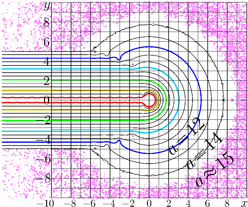 | 800 × 667 (51 KB) | T (talk | contribs) | misprint in the code had been corrected |
| 18:36, 18 January 2026 | 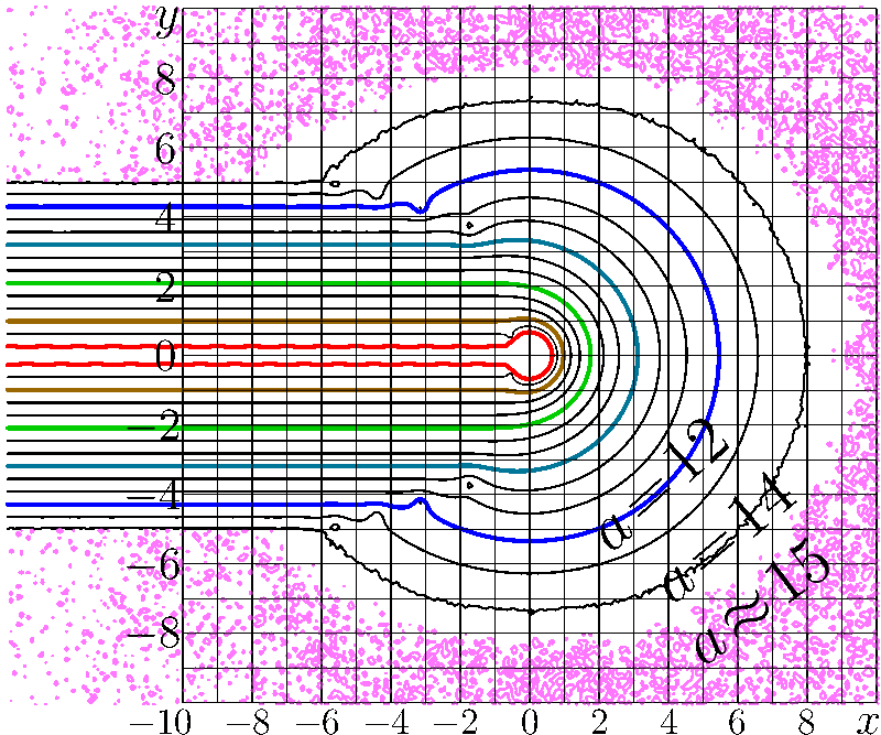 | 800 × 667 (50 KB) | T (talk | contribs) | {{oq|FactoriAsymptoAgreeT.png|Original file (800 × 667 pixels, file size: 50 KB, MIME type: image/png)|400}} Map of agreement \[ a(z) = - \lg \left(\frac {|z!-A(z)|} {|z!|+|A(z)|} \right) \] of the asymptotic \[ A(z)= \sqrt{2\pi z}\ \exp\left(\log\left(\frac{z}{\mathrm e} \right) z + \frac{1}{12 z}\left(1+ \frac{1}{z^2}\left(\frac{-1}{30}+ \frac{1}{z^2}\left(\frac{1}{105}+ \frac{1}{z^2}\left(\frac{-1}{140}+ \frac{1}{z^2}\left(\frac{1}{99}+ \frac{1}{z^2}\left(\frac{-1}{42} \right) \rig... |
You cannot overwrite this file.
File usage
The following page uses this file: