File:FactorialAsymPlotT.png

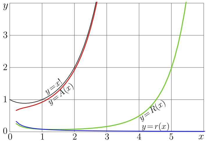
Explicit plot of Factorial and its primitive Stirling asymptotic \[ A(x)=\sqrt{2\pi x} \exp\!\big(\log(x/\mathrm e)\ x\big) \]

The green curve shows he Residual \[ R(x) = x! - A(x) \]

The blue curve shoes the Logarithmic residual \[ r(x) = \log(x!) - \log(A(x)) \] A large \(x\) the residual \( R(x) \) becomes infinite, but \[ \lim_{x\to +\infty} r(x)=0 \] The relation between Factorial and is asymptotic \(A\) can be expressed as follows: \[ f(z) \overset{\log, \ z\in D} {{\underset{ |z|\to \infty}{\huge \sim}}} A(z) \] where \(D\) is arbitrary wide sector that does not include the negative real axis. It can be defined as follows. Let some \(\delta>0\) be fixed. Then, let \[ D\ = \ \big\{ z\!\in\!\mathbb C : \arg(z) < \pi\!-\! \delta \Big\} \] The asymptotic with such a restriction for the phase of the input is restricted asumptoric. More specifically, it can be qualified with term sectorial asymptotic. Many dictionaries and encyclopedias use symbol \(\tilde\) but do not mention that the Stirling formula approach the Factorial within the sector \(D\), that the residual \(R\) diverges but the logarithmic residual \(r\) converges to zero. It is assumed to be obvious for the Stirling asymptotics of Factorial (and those of the Gamma function), but it is not so obvious for asymptotics of more complicated functions.

More precise versions of the Stirling asymptotics provide much better approximations, but they have the same general property: at large values of the input, the Residual \(R\) diverges, but the logarithmic residual \(r\) converges to zero.

C++

#include <math.h>
#include <stdio.h>
#include <stdlib.h>
#define DB double
#define DO(x,y) for(x=0;x<y;x++)
using namespace std;
#include <complex>
typedef complex<double> z_type;
#define Re(x) x.real()
#define Im(x) x.imag()
#define I z_type(0.,1.)
 #include"ado.cin"
 #define M(x,y) fprintf(o,"%6.4f %6.4f M\n",1.*(x),1.*(y));
 #define L(x,y) fprintf(o,"%6.4f %6.4f L\n",1.*(x),1.*(y));
//#include "Conrec6.cin"
#include "fac.cin"
//#include "SuFac.cin"
#include "SuExq2.cin"
//#include "fslog.cin"
//#include "filog.cin"

z_type facas0(z_type z){//  z_type c=1./z; //z_type d=c*c;
return sqrt(M_PI*2.*z)*exp(log(z/M_E)*z
//+(1./12.)*c
//*(1.+d*(-1./30.+d*(1./105.+d*(-1./140.+d*(1./99.+d*(-691./30030.))))))
);}

z_type facas1(z_type z){z_type c=1./z; //z_type d=c*c;
return sqrt(M_PI*2.*z)*exp(log(z/M_E)*z
+(1./12.)*c
//*(1.+d*(-1./30.+d*(1./105.+d*(-1./140.+d*(1./99.+d*(-691./30030.))))))
);}

int main(){ int j,k,m,n; DB x,y, p,q, t; z_type z,c,d;
FILE *o;o=fopen("FactorialAsymPlot.eps","w");ado(o,608,408);
fprintf(o,"4 4 translate\n 100 100 scale\n");

//for(m=0;m<7;m++){M(m,0)L(m,4)}
//for(n=0;n<5;n++){M(0,n)L(6,n)}
fprintf(o,"2 setlinecap\n");

for(m=0;m<40;m++) {x=.0+.1*(m-.03); c=fac(x);  y=Re(c); if(m==0) M(x,y) else L(x,y) if(y>4) break;}
fprintf(o,".016 W 0 0 0 RGB S\n");

for(m=0;m<40;m++) {x=.2+.1*m; c=facas0(x); y=Re(c); if(m==0) M(x,y) else L(x,y) if(y>4) break;}
fprintf(o,".024 W 1 0 0 RGB S\n");

for(m=0;m<60;m++) {x=.2+.1*m; c=fac(x)-facas0(x);  y=Re(c); if(m==0) M(x,y) else L(x,y) if(y>4) break;}
fprintf(o,".03 W 0 .8 0 RGB S\n");

for(m=0;m<60;m++) {x=.2+.1*m; c=log(fac(x))-log(facas0(x));  y=Re(c); if(m==0) M(x,y) else L(x,y) if(y>4) break;}
fprintf(o,".02 W 0 0 1 RGB S\n");

for(m=0;m<7;m++){M(m,0)L(m,4)}
for(n=0;n<5;n++){M(0,n)L(6,n)}
fprintf(o,"2 setlinecap .0012 W 0 0 0 RGB S\n");

fprintf(o,"showpage\n%c%cTrailer",'%','%'); fclose(o);
     system("epstopdf FactorialAsymPlot.eps"); 
     system(    "open FactorialAsymPlot.pdf"); //for mac
}

Latex

\documentclass[12pt]{article}
\usepackage[utf8]{inputenc}
\usepackage[T2A]{fontenc}
\usepackage[russian]{babel}
\usepackage{geometry}
\usepackage{latexsym,amsmath,amssymb,amsbsy,graphicx}
%\usepackage{graphicx}
\usepackage{wrapfig}
\usepackage{hyperref} 
\usepackage{rotating} 
\usepackage[export]{adjustbox}
\paperwidth 640pt
\paperheight 440pt                                                                                                                                                     
\topmargin -114pt
\textheight 740pt
\oddsidemargin -66pt
\textwidth 512pt
\newcommand{\ing}{\includegraphics}
\newcommand{\sx}{\scalebox}
\newcommand{\rot}{\begin{rotate}}
\newcommand{\ero}{\end{rotate}}
\parindent 0px
\begin{document}
%\sx{.82}
{\begin{picture}(640,440)
%\put(20,20){\ing{AteSuFacMap}}
\put(20,20){\ing{FactorialAsymPlot.pdf}}
\put(3,410){\sx{2.7}{\(y\)}}
\put(3,317){\sx{2.5}{\(3\)}}
\put(3,217){\sx{2.4}{\(2\)}}
\put(3,117){\sx{2.4}{\(1\)}}
\put(3,018){\sx{2.4}{\(0\)}}
\put( 19,0){\sx{2.4}{\(0\)}}
\put(119,0){\sx{2.4}{\(1\)}}
\put(219,0){\sx{2.4}{\(2\)}}
\put(319,0){\sx{2.4}{\(3\)}}
\put(419,0){\sx{2.4}{\(4\)}}
\put(519,0){\sx{2.4}{\(5\)}}
%\put(619,0){\sx{2.4}{\(6\)}}
\put(610,1){\sx{2.6}{\(x\)}}
\put(140,141){\sx{2.2}{\rot{37}\(y\!=\!x!\)\ero}} 
\put(150,109){\sx{2.2}{\rot{37}\(y\!=\!A(x)\)\ero}} 

\put(432,59){\sx{2.2}{\rot{34}\(y\!=\!R(x)\)\ero}} 
\put(434,34){\sx{2.2}{\rot{0}\(y\!=\!r(x)\)\ero}} 
\end{picture}}
\end{document}

References

Keywords

«[[]]», «Approximation», «Asymptotic», «Asymptotics», «Factorial», «Logarithnic desoidual», «Residual», «Stirling»,