File:AcoscmapT300.png

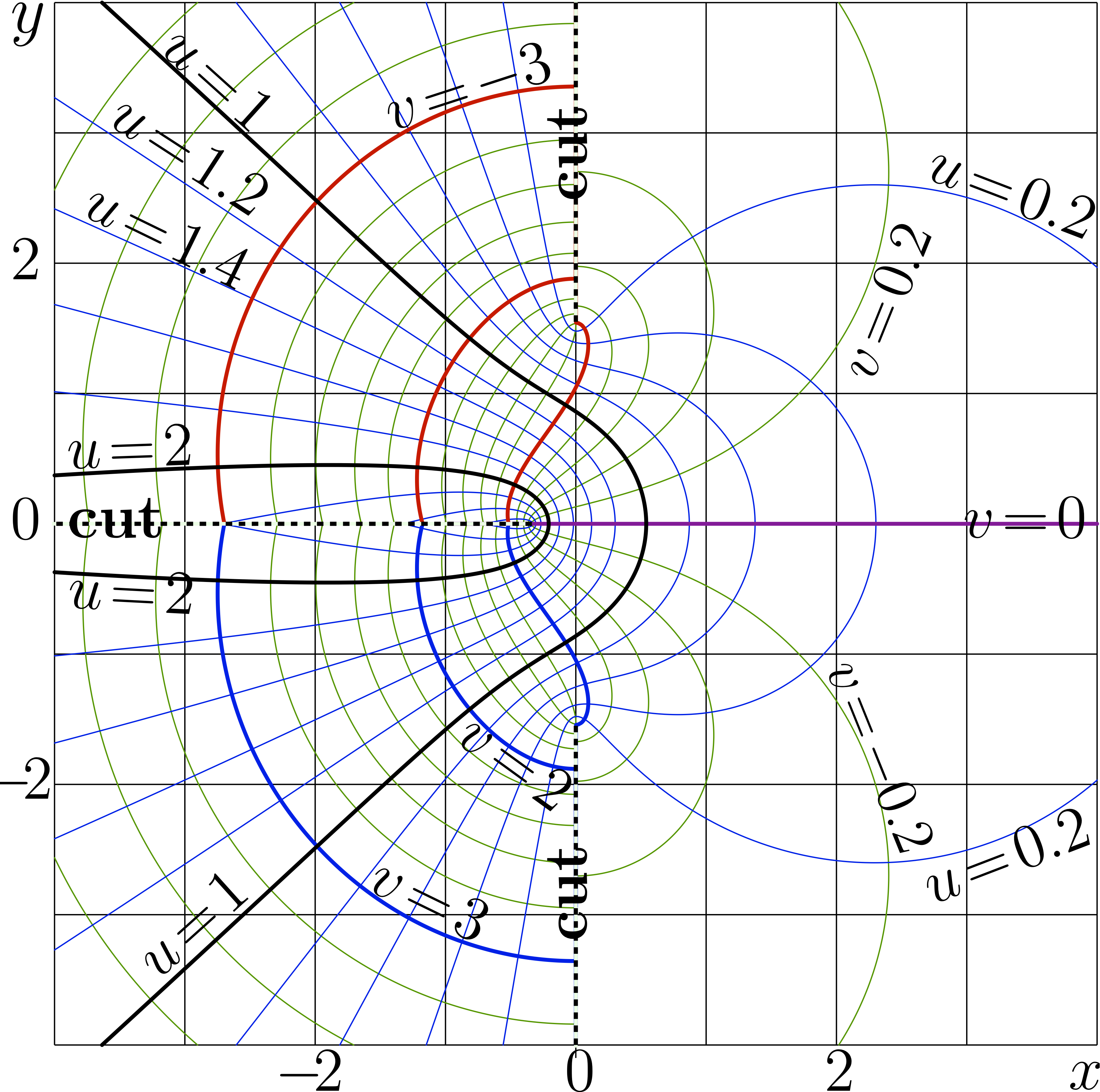
Complex map of function ArcCosc.

C++ generator of curves

For technical reasons, the generator of curves is divided to few sepatated files.

plofu.cin

The code below should be stored as plofu.cin . It determines thickness and color of drawing of lines of constant real part of the function and those for the imaginary part; and also values of these levels. Usually it worth to prepare all the maps in a manuscript in the same style, id est, with the same plofu.cin. However, for different manuscripts and different kinds of functions, the different styles may be required.

fprintf(o,"1 setlinejoin 1 setlinecap\n"); p=1.8;q=.7;
for(m=-11;m<11;m++)for(n=2;n<10;n+=2)conto(o,f,w,v,X,Y,M,N,(m+.1*n),-q, q); fprintf(o,".01 W 0 .6 0 RGB S\n");
for(m=0;m<10;m++) for(n=2;n<10;n+=2)conto(o,g,w,v,X,Y,M,N,-(m+.1*n),-q, q); fprintf(o,".01 W .9 0 0 RGB S\n");
for(m=0;m<10;m++) for(n=2;n<10;n+=2)conto(o,g,w,v,X,Y,M,N, (m+.1*n),-q, q); fprintf(o,".01 W 0 0 .9 RGB S\n");
for(m=1;m<11;m++)  conto(o,f,w,v,X,Y,M,N, (0.-m),-p,p); fprintf(o,".03 W .9 0 0 RGB S\n");
for(m=1;m<11;m++)  conto(o,f,w,v,X,Y,M,N, (0.+m),-p,p); fprintf(o,".03 W 0 0 .9 RGB S\n");
                conto(o,f,w,v,X,Y,M,N, (0.  ),-p,p); fprintf(o,".03 W .6 0 .6 RGB S\n");
for(m=-9;m<10;m++) conto(o,g,w,v,X,Y,M,N, (0.+m),-p,p); fprintf(o,".03 W 0 0 0 RGB S\n");

Evaluation of AcrCosc

The code above is supposed to be stored in the working directory as plofu.cin ; also, files ado.cin and conto.cin should be loaded for the compilation of the code below.

#include <math.h>
#include <stdio.h>
#include <stdlib.h>
#define DB double
#define DO(x,y) for(x=0;x<y;x++)
using namespace std;
#include <complex>
typedef complex<double> z_type;
#define Re(x) x.real()
#define Im(x) x.imag()
#define I z_type(0.,1.)
#include "conto.cin"

z_type cosc(z_type z) {return cos(z)/z;}
z_type cosp(z_type z) {return (-sin(z) - cos(z)/z)/z ;}
z_type cohc(z_type z) {return cosh(z)/z ;}
z_type cohp(z_type z) {return (sinh(z)-cosh(z)/z)/z ;}

z_type acoscL(z_type z){ int n; z_type s,q; z*=-I; q=I*sqrt(1.50887956153832-z);
  s=q*1.1512978931181814 + 1.199678640257734; DO(n,6) s+= (z-cohc(s))/cohp(s);
  return -I*s; }

z_type acoscR(z_type z) {int n; z_type s= (1.-0.5/(z*z))/z;
       DO(n,5) s+=(z-cosc(s))/cosp(s); return s;}

z_type acoscB(z_type z){ z_type t=0.33650841691839534+z, u=sqrt(t), s; int n;
s=    2.798386045783887
+u*(-2.437906425896532
+u*( 0.7079542331649882 
+u*(-0.5009330133042798
+u*( 0.5714459932734446    ))));
DO(n,6) s+=(z-cosc(s))/cosp(s); return s; }

z_type acosc(z_type z){ DB x1=-0.33650841691839534, x=Re(z), y=Im(z), yy=y*y, 
r=x-x1;r*=r;r+=yy; if(r < 1.8 )     return acoscB(z); 
r=x+2.;r*=r;r+=yy; if(r>8. && x>=0) return acoscR(z);
if(y >= 0) return acoscL(z);
      return conj(acoscL(conj(z))); }

main(){ int j,k,m,n; DB x,y, p,q, t; z_type z,c,d;
int M=401,M1=M+1;
int N=401,N1=N+1;
DB X[M1],Y[N1], g[M1*N1],f[M1*N1], w[M1*N1]; // w is working array.
char v[M1*N1]; // v is working array
FILE *o;o=fopen("acoscmap.eps","w");ado(o,82,82);
fprintf(o,"41 41 translate\n 10 10 scale\n");
DO(n,200)Y[n]=-4.+.02*n;
      Y[200]=-.002;
      Y[201]= .002;
for(n=202;n<N1;n++) Y[n]=-4.+.02*(n-1.);
DO(m,M1)X[m]=Y[m];
for(m=-4;m<5;m++){if(m==0){M(m,-4.1)L(m,4.1)} else{M(m,-4)L(m,4)}}
for(n=-4;n<5;n++){     M(  -4,n)L(4,n)}
fprintf(o,".01 W 0 0 0 RGB S\n");
DO(m,M1)DO(n,N1){g[m*N1+n]=9999; f[m*N1+n]=9999;}
DO(m,M1){x=X[m]; //printf("%5.2f\n",x);
DO(n,N1){y=Y[n]; z=z_type(x,y);
       c= acosc(z);
//        d= cosc(c);
//     p=abs((z-d)/(z+d));  p=-log(p)/log(10.);
       p=Re(c);  q=Im(c);        
      if(p>-99. && p<99.
       &&     q>-99. && q<99 
      )
      {g[m*N1+n]=p; 
       f[m*N1+n]=q;
       }
                      }}
// Draw the contours:
// #include "plodi.cin"
 #include "plofu.cin"
// draw the cut lines:
DB x1=-0.33650841691839534;
DB y1= 1.55;
M(-4.02,0)L(x1,0)
M(0,-4.02)L(0,-y1) M(0,y1)L(0,4.02)
fprintf(o,"0 setlinecap .028 W .9 1 .9 RGB S\n");
//
DO(m,37){x=x1-.1*m; M(x,0) L(x-.05,0)}
DO(n,25){y=-y1-.1*n; M(0,y) L(0,y-.05)}
DO(n,25){y=y1+.1*n; M(0,y) L(0,y+.05)}
fprintf(o,".032 W 0 0 0 RGB S\n");

fprintf(o,"showpage\n%c%cTrailer",'%','%'); fclose(o);
      system("epstopdf acoscmap.eps");
      system(    "open acoscmap.pdf");            
      getchar(); system("killall Preview");//for mac
}

Latex generator of labels

File acoscmap.pdf should be generated with the code above in order to compile the latex document below:

%<br> \documentclass[12pt]{article} %<br> \paperheight 838px %<br> \paperwidth 844px %<br> \textwidth 1294px %<br> \textheight 1200px %<br> \topmargin -80px %<br> \oddsidemargin -80px %<br> \usepackage{graphics} %<br> \usepackage{rotating} %<br> \newcommand \sx {\scalebox} %<br> \newcommand \rot {\begin{rotate}} %<br> \newcommand \ero {\end{rotate}} %<br> \newcommand \ing {\includegraphics} %<br> \newcommand \rmi {\mathrm{i}} %<br> \begin{document} %<br> \newcommand \zoomax { %<br> \put(16,820){\sx{4.4}{$y$}} %<br> \put(16,630){\sx{4}{$2$}} %<br> \put(16,430){\sx{4}{$0$}} %<br> \put(-4, 230){\sx{4}{$-\!2$}} %<br> \put(220, 5){\sx{4}{$-\!2$}} %<br> \put(443, 5){\sx{4}{$0$}} %<br> \put(643, 5){\sx{4}{$2$}} %<br> \put(831,6){\sx{4}{$x$}} %<br> } %<br> \parindent 0pt %<br> %\sx{8}{\begin{picture}(86,86) \put(0,0){\ing{b271t0}} %<br> \begin{picture}(816,816) %<br> \put(40,30){\sx{10}{\ing{acoscmap}}} %<br> \zoomax %<br> \put(130,806){\sx{4}{\rot{-42}$u\!=\!1$\ero}} %<br> \put(90,750){\sx{4}{\rot{-33}$u\!=\!1.2$\ero}} %<br> \put(70,680){\sx{4}{\rot{-26}$u\!=\!1.4$\ero}} %<br> \put(60,484){\sx{4}{\rot{2}$u\!=\!2$\ero}} %<br> \put(60,431){\sx{4}{\bf cut}} %<br> \put(460,690){\sx{4}{\rot{90}\bf cut \ero}} %<br> \put(460,120){\sx{4}{\rot{90}\bf cut \ero}} %<br> \put(60,377){\sx{4}{\rot{-3}$u\!=\!2$\ero}} %<br> \put(130,90){\sx{4}{\rot{42}$u\!=\!1$\ero}} %<br> %<br> \put(310,744){\sx{4}{\rot{18}$v\!=\!-3$\ero}} %<br> %\put(370,588){\sx{4}{\rot{34}$v\!=\!-2$\ero}} %<br> \put(358,274){\sx{4}{\rot{-36}$v\!=\!2$\ero}} %<br> \put(290,160){\sx{4}{\rot{-26}$v\!=\!3$\ero}} %<br> %<br> \put(720,708){\sx{4}{\rot{-21}$u\!=\!0.2$\ero}} %<br> \put(750,431){\sx{4}{\rot{00}$v\!=\!0$\ero}} %<br> \put(726,148){\sx{4}{\rot{21}$u\!=\!0.2$\ero}} %<br> %<br> \put(680,550){\sx{3.8}{\rot{68}$v\!=\!0.2$\ero}} %<br> \put(644,330){\sx{3.7}{\rot{-68}$v\!=\!-0.2$\ero}} %<br> %<br> \end{picture} %<br> \end{document} %<br> %

Generation of PNG

PDF file called, for example, AcoscmapT.pdf , henerated with the Latex code above
is converted to PNG format with resolution 300px per inch.

Previous version

This is update of the previous version of this image: http://tori.ils.uec.ac.jp/TORI/index.php/File:AcipmapTpng.png

The algorithm is replaced to the more efficient (simple, fast, robust and precise) numerical implementation of ArcCosc; perhaps, this is final version of the code.