File:ArcYulyaPlot100.png

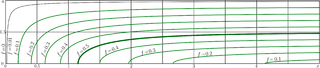
Contour plot of function inverse of the Yulya function, $\mathrm{ArcYulya}\!=\!\mathrm{ArcYulya}^{-1}$.

Levels of constant $f\!=\!\mathrm{ArcYulya}_a(x)$ are shown in the $x,a$ plane.

Generator of curves

Files conto.cin and ado.cin should be stored in the working directory in order to compile the C++ code below:

#include <math.h>
#include <stdio.h>
#include <stdlib.h>
#define DB double
#define DO(x,y) for(x=0;x<y;x++)
using namespace std;

DB Yulya(DB a, DB x){ DB p=a+x; DB m=a-x; 
     return p/sqrt(1.-p*p)-m/sqrt(1.-m*m);}

DB Yulyap(DB a, DB x){ DB p,m; p=a+x; m=a-x; p=1.-p*p; m=1.-m*m; 
     return 1./(p*sqrt(p))+1./(m*sqrt(m));}

DB ArcYulya0(DB a, DB f){ DB m=1.-a; DB p=1.+a; 
         return m*f / sqrt( 4./(m*p*p*p) + f*f );}

DB ArcYulya2(DB a, DB f){ DB y=ArcYulya0(a,f);
        y+=(f-Yulya(a,y))/Yulyap(a,y);
        y+=(f-Yulya(a,y))/Yulyap(a,y);
        y+=(f-Yulya(a,y))/Yulyap(a,y);
        y+=(f-Yulya(a,y))/Yulyap(a,y);
        return y;}

#include "conto.cin"
main(){ int j,k,m,n; DB x,y, p,q, t;
int M=501,M1=M+1;
int N=201,N1=N+1;
DB X[M1],Y[N1], g[M1*N1], w[M1*N1]; // w is working array.
char v[M1*N1]; // v is working array
FILE *o;o=fopen("arcyulya.eps","w");ado(o,508,108);
fprintf(o,"4 4 translate\n 100 100 scale\n");
DO(m,M1) X[m]=0. +.01*(m-.5);
DO(n,N1) Y[n]=0. +.005*(n-.1);
for(m=0;m<51;m+=5){     M(.1*m,0) L(.1*m,1)}
for(n=0;n<11;n+=5){     M(0,.1*n)L(5,.1*n)}
fprintf(o,".006 W 0 0 0 RGB S\n");
DO(m,M1)DO(n,N1){g[m*N1+n]=9999;}
DO(m,M1){x=X[m]; //printf("run at x=%6.3f\n",x);
DO(n,N1){y=Y[n];
        p=x*x+y*y;
        p=ArcYulya2(y,x);
        if(p>-85 && p<85)  g[m*N1+n]=p;
        }}
 fprintf(o,"1 setlinejoin 1 setlinecap\n");
p=2.; 
conto(o,g,w,v,X,Y,M,N,.01,-p,p);fprintf(o,".005 W 0 0 0 RGB S\n");
conto(o,g,w,v,X,Y,M,N,.1,-p,p);fprintf(o,".01 W 0 .5 0 RGB S\n");
conto(o,g,w,v,X,Y,M,N,.2,-p,p);fprintf(o,".01 W 0 .5 0 RGB S\n");
conto(o,g,w,v,X,Y,M,N,.3,-p,p);fprintf(o,".01 W 0 .5 0 RGB S\n");
conto(o,g,w,v,X,Y,M,N,.4,-p,p);fprintf(o,".01 W 0 .5 0 RGB S\n");
conto(o,g,w,v,X,Y,M,N,.5,-p,p);fprintf(o,".02 W 0 .4 0 RGB S\n");
conto(o,g,w,v,X,Y,M,N,.6,-p,p);fprintf(o,".01 W 0 .5 0 RGB S\n");
conto(o,g,w,v,X,Y,M,N,.7,-p,p);fprintf(o,".01 W 0 .5 0 RGB S\n");
conto(o,g,w,v,X,Y,M,N,.8,-p,p);fprintf(o,".01 W 0 .5 0 RGB S\n");
conto(o,g,w,v,X,Y,M,N,.9,-p,p);fprintf(o,".01 W 0 .5 0 RGB S\n");
fprintf(o,"showpage\n%cTrailer",'%'); fclose(o);
        system("epstopdf arcyulya.eps");
        system(    "open arcyulya.pdf"); //these 2 commands may be specific for macintosh
getchar(); system("killall Preview");// if run at another operational sysetm, may need to modify
}
//Copyleft 2011 by Dmitrii Kouznetsov

Generator of lables

The latex document below includes the arcyulya.pdf generated in the previous section and add the lables. The result is converted to the png format.

\documentclass[12pt]{article} %<br> \usepackage{geometry} %<br> \usepackage{graphicx} %<br> \usepackage{rotating} %<br> \paperwidth 2558pt %<br> \paperheight 540pt %<br> \topmargin -114pt %<br> \oddsidemargin -100pt %<br> \textwidth 2600pt %<br> \textheight 600pt %<br> \pagestyle {empty} %<br> \newcommand \sx {\scalebox} %<br> \newcommand \rot {\begin{rotate}} %<br> \newcommand \ero {\end{rotate}} %<br> \newcommand \ing {\includegraphics} %<br> \begin{document} %<br> \sx{5}{ \begin{picture}(508,108) %<br> \put(3,2){\ing{arcyulya}} %<br> \put(1,103){\sx{.7}{$a$}} %<br> \put(-2,54){\sx{.6}{$0.5$}} %<br> \put(0,4){\sx{.6}{$0$}} %<br> \put(5,0){\sx{.6}{$0$}} %<br> \put(53,0){\sx{.6}{$0.5$}} %<br> \put(106,0){\sx{.66}{$1$}} %<br> \put(206,0){\sx{.66}{$2$}} %<br> \put(306,0){\sx{.66}{$3$}} %<br> \put(406,0){\sx{.66}{$4$}} %<br> \put(504,0){\sx{.7}{$x$}} %<br> \put(6,20){\rot{90} \sx{.7}{$f\!=\!0$} \ero} %<br> \put(16,20){\rot{88} \sx{.7}{$f\!=\!0.01$} \ero} %<br> \put(26,19){\rot{82} \sx{.7}{$f\!=\!0.1$} \ero} %<br> \put(46,17){\rot{73} \sx{.7}{$f\!=\!0.2$} \ero} %<br> \put(68,17){\rot{64} \sx{.7}{$f\!=\!0.3$} \ero} %<br> \put(93,17){\rot{55} \sx{.7}{$f\!=\!0.4$} \ero} %<br> \put(123,18){\rot{40} \sx{.7}{$f\!=\!0.5$} \ero} %<br> \put(166,21){\rot{22} \sx{.7}{$f\!=\!0.4$} \ero} %<br> \put(224,20){\rot{13} \sx{.7}{$f\!=\!0.3$} \ero} %<br> \put(314,18){\rot{4} \sx{.7}{$f\!=\!0.2$} \ero} %<br> \put(424,10){\rot{3} \sx{.7}{$f\!=\!0.1$} \ero} %<br> \end{picture} %<br> } %<br> \end{document}

Testing of the implementaitons of Yulya and ArcYulya

For the testing, the following two quantities should be plotted in the $x,a$ coordinates:

Yulya(a,ArcYulya2(a,x))-x

ArcYulya2(a,Yulya(a,x))-x

Permission to reuse

Copleft 2011 by Dmitrii Kouznetsov. The image and its generators may be used for free, attribute the source.