File:GammaAsymptoBgreeT.png

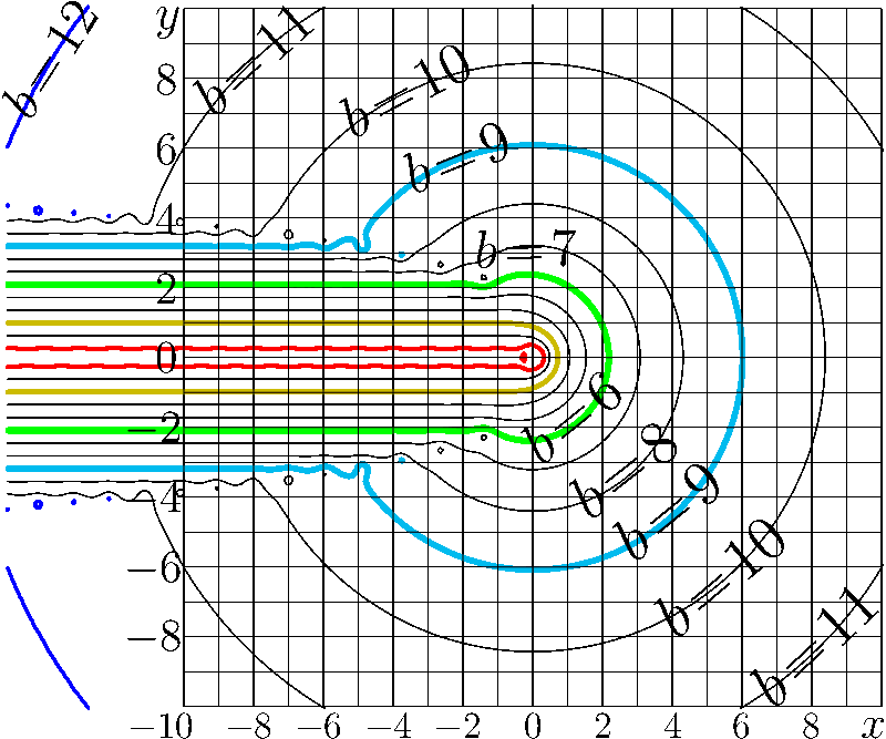
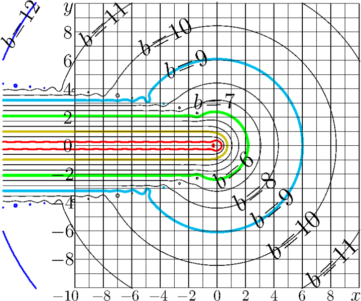
Agreement of Gamma function (implemented through the Factorial from fac.cin) with its asymptotic by ^[1] (forula 5.11.3), (year 2026) : \[ \Gamma(z) \sim \mathrm e^{-z} z^z \left(\frac{2\pi}{z}\right)^{1/2} \sum_{k=0}^{\infty} \frac{g_k}{z^k} \]

Surprisly for Editor, the coefficients \(g\) happen to be the same as the coefficient in the similar asymptotic expansion for the Factorial; so, they are not repeated in the code below.

The asymptotic \(B\) is taken from the expansion above; the series is truncated keeping the last term \(\sim 1/z^6\).

The agreement \(b\) is defined \[ b(z) = - \lg \left(\frac{|\Gamma(z)-B(z)|}{|\Gamma(z)|+|B(z)|}\right). \]

In the picture, \(b(x-\mathrm i y)\) is shown with contour lines in the \(x,y\) plane.

C++ code

// c++ -std=c++11 GammaAsymptoBgree.cc -O2 -o GammaAsymptoBgree
#include <math.h>
#include <stdio.h>
#include <stdlib.h>
#define DB double
#define DO(x,y) for(x=0;x<y;x++)
using namespace std;
#include <complex>
typedef complex<double> z_type;
#define Re(x) x.real()
#define Im(x) x.imag()
#define I z_type(0.,1.)
#include"ado.cin"
#define M(x,y) fprintf(o,"%6.4f %6.4f M\n",1.*(x),1.*(y));
#define L(x,y) fprintf(o,"%6.4f %6.4f L\n",1.*(x),1.*(y));
#include "Conrec6.cin"
#include "fac.cin"

z_type facas(z_type z){ z_type c=1./z; z_type d=c*c;
return sqrt(M_PI*2.*z)*exp(log(z/M_E)*z+
(1./12.)*c*(
1.+d*(-1./30.+d*(1./105.+d*(-1./140.+d*(1./99.+d*(-691./30030.)))))
));
}

z_type gamc(z_type z){  z_type t=1./z; z_type s; int n;
DB c[12] = { 1.,
 0.083333333333333329,
 0.003472222222222222,
-0.002681327160493827,
-0.000229472093621399,
 0.000784039221720067,
 0.000069728137583659,
 0.,
 0.,
 0.,
 0.,
 0.,};
c[7]=-.00059225;c[8]=-.0000515; c[9]=0.000836; c[10]= .00011; c[11]=-.0001;//23
int N=6;
s=c[N]*t;
for(n=N-1;n>0;n--){s+=c[n];s*=t;}
return sqrt(2*M_PI/z)*exp(log(z/M_E)*z)*(s+1.);
}

int main(){ int j,k,m,n; DB x,y, p,q, t; z_type z,c,d;
int M=251,M1=M+1;
int N=201,N1=N+1;
DB X[M1],Y[N1], g[M1*N1];
//,f[M1*N1];
FILE *o;o=fopen("GammaAsymptoBgree.eps","w");ado(o,252,202);
fprintf(o,"151 101 translate\n 10 10 scale\n");

//fprintf(o,"0 0 0 13 0 360 arc .5 W 0 1 1 RGB S\n");
//fprintf(o,"0 0 0 10 0 360 arc .5 W 0 1 1 RGB S\n");

DO(m,M1) X[m]=-15+.1*(m-.5);
DO(n,N1) Y[n]=-10+.1*(n-.5);

DO(m,M1)DO(n,N1){g[m+M1*n]=9999;}
DO(m,M1){x=X[m]; //printf("%5.2f\n",x);
DO(n,N1){y=Y[n]; z=z_type(x,y); 
// c=Filog(z);
//c=z*z*sin(1./z);
//c=fac(z);
c=fac(z-1.); // it is supposed to be Gamma(z) ..
d=gamc(z); // it is asymptotic of Gamma by https://dlmf.nist.gov/5.11
//d=facas(z);
p= - log( abs(c-d) / (abs(c)+abs(d)) )/log(10.);
//p=Re(c);q=Im(c); 
g[m+M1*n]=p;
       }}
fprintf(o,"1 setlinejoin 1 setlinecap\n"); p=5.;q=1;
p=15.;
Conrec6(o,g,X,Y,M1,N1, 1. ,p); fprintf(o,".12 W 1 0 0 RGB S\n");
Conrec6(o,g,X,Y,M1,N1, 2. ,p); fprintf(o,".04 W 0 0 0 RGB S\n");
Conrec6(o,g,X,Y,M1,N1, 3. ,p); fprintf(o,".14 W .8 .7 0 RGB S\n");
Conrec6(o,g,X,Y,M1,N1, 4. ,p); fprintf(o,".04 W 0 0 0 RGB S\n");
Conrec6(o,g,X,Y,M1,N1, 5. ,p); fprintf(o,".04 W 0 0 0 RGB S\n");
Conrec6(o,g,X,Y,M1,N1, 6. ,p); fprintf(o,".18 W 0 8 0 RGB S\n");
Conrec6(o,g,X,Y,M1,N1, 7. ,p); fprintf(o,".04 W 0 0 0 RGB S\n");
Conrec6(o,g,X,Y,M1,N1, 8. ,p); fprintf(o,".04 W 0 0 0 RGB S\n");
Conrec6(o,g,X,Y,M1,N1, 9. ,p); fprintf(o,".17 W 0 .7 .9 RGB S\n");
Conrec6(o,g,X,Y,M1,N1, 10. ,p); fprintf(o,".04 W 0 0 0 RGB S\n");
Conrec6(o,g,X,Y,M1,N1, 11. ,p); fprintf(o,".04 W 0 0 0 RGB S\n");
Conrec6(o,g,X,Y,M1,N1, 12. ,p); fprintf(o,".10 W 0 0 1 RGB S\n");
Conrec6(o,g,X,Y,M1,N1, 13. ,p); fprintf(o,".04 W 0 0 0 RGB S\n");
Conrec6(o,g,X,Y,M1,N1, 14. ,p); fprintf(o,".04 W 0 0 0 RGB S\n");
Conrec6(o,g,X,Y,M1,N1, 15. ,p); fprintf(o,".07 W 1 .5 1 RGB S\n");

for(m=-10;m<11;m++){if(m!=0){M(m,-10)L(m,10)}}
for(n=-10;n<11;n++){M(-10,n)L(10,n)}
fprintf(o,"2 setlinecap .02 W 0 0 0 RGB S\n");
fprintf(o,"2 setlinecap .02 W 0 0 0 RGB S\n");
M(0,-10)L(0,11)
fprintf(o,"2 setlinecap .03 W 0 0 0 RGB S\n");

fprintf(o,"showpage\n%c%cTrailer",'%','%'); fclose(o);
     system("epstopdf GammaAsymptoBgree.eps"); 
     system(    "open GammaAsymptoBgree.pdf"); //for mac

Latex

\documentclass[12pt]{article}
\usepackage{geometry}
\paperwidth 803pt
\paperheight 669pt
\textwidth 800pt
\textheight 700pt
\topmargin -106pt
\oddsidemargin -116pt
\usepackage{graphicx}
\usepackage{rotating}
\newcommand \rot {\begin{rotate}}
\newcommand \ero {\end{rotate}}
\newcommand \rme {\mathrm{e}}
\newcommand \sx {\scalebox}
\begin{document}
\sx{3.15}{\begin{picture}(230,211)
\normalsize
%\put(10,10){\includegraphics{Z2sin1zMap}}
%\put(10,8){\includegraphics{FactoriAsymptoAgree}}
\put(10,8){\includegraphics{GammaAsymptoBgree}}
\put(53,204){\sx{1.2}{\(y\)}}
\put(53,185){\sx{1.1}{\(8\)}}
\put(53,165){\sx{1.1}{\(6\)}}
\put(53,145){\sx{1.1}{\(4\)}}
\put(53,125){\sx{1.1}{\(2\)}}
\put(53,105){\sx{1.1}{\(0\)}}
\put(44,85){\sx{1.1}{\(-2\)}}
\put(44,65){\sx{1.1}{\(-4\)}}
\put(44,45){\sx{1.1}{\(-6\)}}
\put(44,25){\sx{1.1}{\(-8\)}}
\put(45, 0){\sx{.9}{\(-10\)}}
\put(73, 0){\sx{.9}{\(-8\)}}
\put(93, 0){\sx{.9}{\(-6\)}}
\put(113, 0){\sx{.9}{\(-4\)}}
\put(133, 0){\sx{.9}{\(-2\)}}
\put(159, 0){\sx{.9}{\(0\)}}
\put(179, 0){\sx{.9}{\(2\)}}
\put(199, 0){\sx{.9}{\(4\)}}
\put(219, 0){\sx{.9}{\(6\)}}
\put(239, 0){\sx{.9}{\(8\)}}
\put(256, 0){\sx{1.1}{\(x\)}}
\put(17,177){\sx{1.3}{\rot{57}\(b\!=\!12\) \ero} }
\put(70,178){\sx{1.4}{\rot{42}\(b\!=\!11\) \ero} }
\put(110,172){\sx{1.4}{\rot{28}\(b\!=\!10\) \ero} }
\put(127,156){\sx{1.4}{\rot{22}\(b\!=\!9\) \ero} }
%\put(141,144){\sx{1.4}{\rot{9}\(b\!=\!8\) \ero} }
\put(145,135){\sx{1.3}{\rot{2}\(b\!=\!7\) \ero} }
%\put(132,196){\sx{1.6}{\rot{0}\(a\!\approx\!15\) \ero} }
%\put(132,176){\sx{1.6}{\rot{0}\(a\!=\!14\) \ero} }
%\put(132,156){\sx{1.6}{\rot{0}\(a\!=\!12\) \ero} }

\put(164,78){\sx{1.4}{\rot{39}\(b\!=\!6\) \ero} }
\put(178,62){\sx{1.5}{\rot{38}\(b\!=\!8\) \ero} }
\put(191,50){\sx{1.5}{\rot{39}\(b\!=\!9\) \ero} }
\put(203,28){\sx{1.5}{\rot{40}\(b\!=\!10\) \ero} }
\put(231,8){\sx{1.5}{\rot{43}\(b\!=\!11\) \ero} }
%\put(203,37){\sx{1.6}{\rot{42}\(b\!=\!14\) \ero} }
%\put(212,19){\sx{1.6}{\rot{37}\(b\!\approx\!15\) \ero} }
\end{picture}}
\end{document} 

Notes

The series in the original definition seem to diverge, as the Bernoulli numbers do not decay.

In TORI, the Gamma function and ArcGamma) are implemented through the Factorial (see fac.cin) and the ArcFactorial. This implementation is historic, see «Square root of factorial».

The questions wether Gamma function is easier to implement than Factorial is under investigation.

The code above is designed to see, how sensitive is the result with respect to the precision of evaluation of the coefficients \(g\).
The algorithm seems to be pretty stable with respect to these coefficients. In this, nothing interesting is found, so, this part of the research is not described here; the code is not modified in order to avoid additional mistakes.

But there exist another interesting observation about this expansion.

The Latex code happens to be almost the same as in the asymptotic of the Factorial; the pictures also look just the same.

This property was unexpected for Editor.

References

Keywords

«ado.cin», «fac.cin», «Conrec6.cin», «AbramowitzStegun», «Asymtotic», «Gamma function», «Factorial», «Restricted asymtotic», «Stirling», «WhittakerWatson»,

References

- ↑ https://dlmf.nist.gov/5.11 About the Project 5 Gamma Function .. The expansion (5.11.1) is called Stirling’s series (Whittaker and Watson (1927, §12.33)), whereas the expansion (5.11.3), or sometimes just its leading term, is known as Stirling’s formula (Abramowitz and Stegun (1964, §6.1), Olver (1997b, p. 88)).