Student Distribution

\(y=\mathrm{Student}(n,x)\) for \(n\!= 1,2,3,4,5,\infty \)

\( u+\mathrm i v = \mathrm{Student}(5, x+\mathrm i y)\)

  \( u+\mathrm i v = \mathrm{Student}(\infty, x+\mathrm i y)\)

Student Distribution is term from scientific slang; it may refer to hololomorphic function of two variables

\(\displaystyle \mathrm{Student}(\nu,t) =\mathrm{Student}_\nu(t) = \) \(\displaystyle \frac{\Gamma\left(\frac{\nu+1}{ 2 }\right)}{\sqrt{\pi\ \nu}\ \Gamma\left(\frac{\nu}{2}\right)} \left(1 + \frac{~ t^2}{\nu }\right)^{-(\nu+1)/2}\)

Here \(\Gamma\) refers to Gamma function, \(\Gamma(z)\) \(=\) Factorial\((z\!-\!1)\) .

In TORI, the Factorial is implemented better than the Gamma function, so,

\(\displaystyle \mathrm{Sturent}(\nu,t) = \) \(\displaystyle \frac{\mathrm{Factorial}\left(\frac{\nu-1}{2}\right)}{\sqrt{\pi\ \nu}\ \mathrm{Factorial}\left(\frac{\nu}{2}-1\right)} \left(1+\frac{t^2}{\nu}\right)^{-(\nu+1)/2}\)

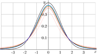
For integer values of the first argument and real values of the second argument, Function \(\mathrm{Student}\) is shown in figure above.

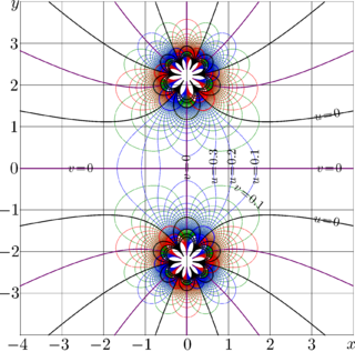
The complex map for \(\nu=5\) is shown in figure at right.

The more official, rigorous (and not so easy to handle) name for the Student Distribution is «Probability density of the Student's t-distribution».
This article uses copipasts from https://en.wikipedia.org/wiki/Student%27s_t-distribution .

Ctudent

Integral of the Student Distriution with respect to the second argument may be referred as Student Cumulative, or Ctudent, or, more formally, «Cumulative Student distribution function»;

\(\displaystyle \mathrm{Ctudent}(\nu,t) = \int_{-\infty}^t \mathrm{Student}(\nu,x) \mathrm{d} x \)

It can be expressed through the Incomplete beta function or though the Hypergeometric function. Up to year 2024, none of these two functions is implemented at TORI.

Editor did not find any convenient and usual notations for functions Student and Ctudent; in future, names Student and Ctudent may be replaced to something more suitable and convenient.

Special cases

Wikipedia suggests simple expressions for the first 5 Students and Ctudents.
The table is reproduced below.
Names «Student» and «Ctudent» are added in search for the best notations.

\(\ \nu\ \)	PDF: \(\mathrm{Student}_\nu(t)\)	CDF: \(\mathrm{Ctudent}_\nu(t)\)	See also
1	\(\ \frac{\ 1\ }{\ \pi\ (1 + t^2)\ }\ \)	\(\ \frac{\ 1\ }{ 2 } + \frac{\ 1\ }{ \pi }\ \arctan(\ t\ )\ \)	Cauchy distribution
2	\(\ \frac{ 1 }{\ 2\ \sqrt{2\ }\ \left(1+\frac{t^2}{2}\right)^{3/2}}\ \)	\(\ \frac{ 1 }{\ 2\ }+\frac{ t }{\ 2\sqrt{2\ }\ \sqrt{ 1 + \frac{~ t^2\ }{ 2 }\ }\ }\ \)
3	\(\ \frac{ 2 }{\ \pi\ \sqrt{3\ }\ \left(\ 1 + \frac{~ t^2\ }{ 3 }\ \right)^2\ }\ \)	\(\ \frac{\ 1\ }{ 2 } + \frac{\ 1\ }{ \pi }\ \left[ \frac{ \left(\ \frac{ t }{\ \sqrt{3\ }\ }\ \right) }{ \left(\ 1 + \frac{~ t^2\ }{ 3 }\ \right) } + \arctan\left(\ \frac{ t }{\ \sqrt{3\ }\ }\ \right)\ \right]\ \)
4	\(\ \frac{\ 3\ }{\ 8\ \left(\ 1 + \frac{~ t^2\ }{ 4 }\ \right)^{5/2}}\ \)	\(\ \frac{\ 1\ }{ 2 } + \frac{\ 3\ }{ 8 } \left[\ \frac{ t }{\ \sqrt{ 1 + \frac{~ t^2\ }{ 4 } ~}\ } \right] \left[\ 1 - \frac{~ t^2\ }{\ 12\ \left(\ 1 + \frac{~ t^2\ }{ 4 }\ \right)\ }\ \right]\ \)
5	\(\ \frac{ 8 }{\ 3 \pi \sqrt{5\ }\left(1+\frac{\ t^2\ }{ 5 }\right)^3\ }\ \)	\(\ \frac{\ 1\ }{ 2 } + \frac{\ 1\ }{\pi}{ \left[ \frac{ t }{\ \sqrt{5\ }\left(1 + \frac{\ t^2\ }{ 5 }\right)\ } \left(1 + \frac{ 2 }{\ 3 \left(1 + \frac{\ t^2\ }{ 5 }\right)\ }\right) + \arctan\left( \frac{ t }{\ \sqrt{\ 5\ }\ } \right)\right]}\ \)
\(\ \infty\ \)	\(\ \frac{ 1 }{\ \sqrt{2 \pi\ }\ }\ e^{-t^2/2}\)	\(\ \frac{\ 1\ }{ 2 }\ {\left[ 1 + \operatorname{erf}\left( \frac{ t }{\ \sqrt{2\ }\ } \right) \right]}\ \)	Normal distribution, Error function

C++ implementation

Usually, the Student Distribution appears with integer (and not so big) values of the first argument ( let it be \(n\)) and real values of the second argument (let it he \(x)\).

For this case with \(0<n<11\), the implementation Student.cin is suggested; it is repeated below.

float Student(int n,float x)
{float c[11]={0.,
0.31830988618379,
0.35355339059327,
0.36755259694786,
0.37500000000000,
0.37960668982249,
0.38273277230987,
0.38499145083227,
0.38669902096139,
0.38803490887167,
0.38910838396603};
return c[n]*pow(1.+x*x/n, -0.5*(n+1));
}

For \(n>10\), the Gaussian distribution is recommended instead of the Student Distribution. In most of cases, there is no need to use a sledgehammer to crack a nut (as it is shown in figure at right). The following relation takes place:

\(\displaystyle \mathrm{Student}(\infty,x) = \mathrm{Gau}(x)= \frac{\exp(-z^2/2)}{\sqrt\pi} \)

The implementation above evaluates the density of the Student Distribution for real values of the argument. However the case of complex argument is also not a big deal.

As the Factorial function is already implemented, the complex double implementation of the Student Distribution is straight forward for complex values of the arguments. That implementation had been used to evaluate the array of coefficients in the code above.

Application

Large number of data

The Student Distribution is basic tool at the statistical analysis of experimental data, when some value is measured many times, and the errors at the measurement are supposed to be independent and have the Gaussian distribution.

Roughly, if some quantity is measured \(N\) times, and values \(a_n\) are obtained, with \(n\) from \(1\) to \(N\)
then the quantity is estimated to be

\( \displaystyle a_0 = \frac{1}{N} \sum_{n=1}^N a_n \)

and the «expected error», «possible deviation» of this estimate from some «true value», in its turn, is estimated as

\( \displaystyle D = \sqrt{\frac{1}{(N\!-\!1) (N\!-\!3)} \sum_{n=1}^N (a_n-a_0)^2} \)

At large \(N\), the error of estimates \(А\), id est, \(a_0-A\) is supposed to have the Gaussian distribution. Assuming this, the colleagues actually use the \(\mathrm{Student}_\infty \) without to mention it.

Mean-square deviation

At small \(N\), the peak of the density of distribution of deviations of \(A\) from the true value is sharper and have wide "wings", than the Gaussian at the same mean-scare deviation; for \(N=2\) and \(N=3\), the mean-square deviation is not defined as a real number.

The Student Distribution has sense for the analysis or rare phenomena, when new, more accurate measurement happens to be far away from the expected «Gaussian». The new value may happen to be still at the tail of the Student Distribution.

In the primitive approach, to show the statistical significance of the estimate, instead of the Gaussian bell, the Srudent distribution of the same width should be iused; the first parameter \( \nu=N-1 \), where \(N\) is number or independent measurements performed.

For \(N\) measurements, the distribution of the averaged results can be expressed with function \(\mathrm{Student}_{N-1} \)

For the Student distribution, the variance

\(\displaystyle V_n=\int_{-\infty}^{\infty} \mathrm{Student}(n,x) \ x^2 \mathrm d x = \frac{n}{n-2} \)

with \( n = N\!-\!1 \).

The mean square deviation is

\( \displaystyle S_n = \sqrt{V_n}=\sqrt{\frac{n}{n\!-\!2}}=\sqrt{\frac{N\!-\!1}{N\!-\!3}} \)

At least 4 measurements (\(n\!=\!3\) , \(N\!=\!4\)) are necessary in order to characterize, how close to the «true value» \(A\) the estimate \(a_0\) is expected to happen, in terms of the mean-square deviation.

Advanced

The less data one has, the more advanced formalism should be applied to use them well.

Let     \( \displaystyle q = \frac{1}{N\!-\!1} \sum_{m=1}^{N} (a_m - a_0)^2 \)

Then, quantity     \( \displaystyle t=\frac{a_0-A}{\sqrt{q/N}} \)

is distributed according to a Student's t-distribution with     \(n=N-1\) degrees of freedom.

Letter t, used as the identifier above, happen to be part of the full name «Student's t-distribution density».

In such a way, instead of the bell \(\mathrm{Gau}\), the \(\mathrm{Student}_{N-1} \) should be used.

This authentically takes into account the spreading of the mean-square deviation in compare to the Gaussian.

This is the main reason not to adjust the second moment of the Student Distribution; for this reason, namely Student function (and not the «scaled Student») is used.

The resulting bell    

\(\displaystyle F(x)=\mathrm{Student}_{N-1}\!\left( \frac{x-a_0}{\sqrt{q/N}} \right) \frac{1}{\sqrt{q/N}} \)

characterizes the precision of approximation of the «true value» \(A\) with estimate \(a_0\).

Collecting the notations above, it can be written as follows:

\(\displaystyle F(x)=\mathrm{Student}_{N-1}\left( \frac{x-a_0}{\sqrt{\frac{1}{\displaystyle(N\!-\!1) N} \sum_{m=1}^{N} (a_m - a_0)^2}} \right) \frac{1}{\displaystyle{\sqrt{\frac{1}{(N\!-\!1) N} \sum_{m=1}^{N} (a_m - a_0)^2}}} \)

or even

\(\displaystyle F(x)=\mathrm{Student}_{N-1}\left( (x-a_0) \sqrt{ \frac{(N\!-\!1) N} { \sum_{m=1}^{N} (a_m - a_0)^2} } \right) \sqrt{ \frac{(N\!-\!1) N} { \sum_{m=1}^{N} (a_m - a_0)^2} } \)

At the slang of physicists, function \(F(x)\) is considered as probability density, that the «true value» \(A\) happens to be \(x\).

Such an approach is practical and easy to interpret .
More correctly, function \(F\) above should be called "Likelihood density", to avoid confusion with probability.

For the Student Distribution, the variance

\( \displaystyle V_n=\int_{-\infty}^{\infty} \mathrm{Student}_n(x) \ x^2 \ \mathrm d x = \frac {n}{n-2} \)

with \(n\!=\!N\!-\!1\) , quantity

\(\displaystyle V_n=\sqrt{ \frac { \sum_{m=1}^{N} (a_m - a_0)^2} {(N\!-\!3)\ N} } \)

can be treated as a «mean-square error of the evaluation of quantity \(A\) with set of \(N\) independent measurements».

\(V_n\) can be interpreted also as «The mean square deviation» of evaluated \(a_0\) from the «true value» \( A \). However, it assumes that \(N\) is integer and \(\ N\!>\!3 \ \) .

References

Keywords

«[[]]», «Density of probability», «Probability», «Student Distribution»,