Difference between revisions of "File:KellerPlotT.png"
($ -> \( ; refs ; add fig) |
(→Latex generator of labels: pre) |
||
| Line 58: | Line 58: | ||
% File [[KellerPlot.pdf]] should be generated with the code above in order to compile the [[Latex]] document below. |
% File [[KellerPlot.pdf]] should be generated with the code above in order to compile the [[Latex]] document below. |
||
| − | %< |
+ | %<pre> |
\documentclass[12pt]{article} %<br> |
\documentclass[12pt]{article} %<br> |
||
\usepackage{geometry} %<br> |
\usepackage{geometry} %<br> |
||
Latest revision as of 09:36, 19 August 2025

Explicit plot of various iterations \(t\) the Keller function.
\( y=\mathrm{Keller}^t(x)=\mathrm{Shoka}\Big( t + \mathrm{ArcShoka}(x)\Big) \)
See more detailed map at right (for non-integer iterates)
To plot this graphic, the iterates of the Keller function are implemented through the Shoka function and the ArcShoka function.
The detailed map is used as Fig.5.11 at page 56 of book «Superfunctions»[1][2].
C++ generator of curves]]
// File ado.cin shold be loaded in order to compile the C++ code below.
 #include <math.h>
 #include <stdio.h>
 #include <stdlib.h>
 #define DB double
 #define DO(x,y) for(x=0;x<y;x++)
 using namespace std;
 #include <complex>
 typedef complex<double> z_type;
 #define Re(x) x.real()
 #define Im(x) x.imag()
 #define I z_type(0.,1.)

 #include"ado.cin"

 z_type Shoka(z_type  z)  { return z + log(exp(-z)+(M_E-1.)); }
 z_type ArcShoka(z_type z){ return z + log((1.-exp(-z))/(M_E-1.)) ;}

 #define M(x,y) fprintf(o,"%6.3f %6.3f M\n",0.+x,0.+y);
 #define L(x,y) fprintf(o,"%6.3f %6.3f L\n",0.+x,0.+y);
 main(){ int j,k,m,n; DB x,y, a;
 FILE *o;o=fopen("KellerPlot.eps","w");ado(o,408,412);
 fprintf(o,"4 4 translate\n 100 100 scale 2 setlinecap 1 setlinejoin\n");
 for(m=0;m<5;m++){ M(m,0)L(m,4)}
 for(n=0;n<5;n++){ M(0,n)L(4,n)}
 M(0,0)L(4,4)
 fprintf(o,".01 W 0 0 0 RGB S\n");
 DO(n,134){x=.005+.01*n;y=Re(Shoka(3.+ArcShoka(x)));if(n==0)M(x,y)else L(x,y)} fprintf(o,".02 W 0 0 .5 RGB S\n");
 DO(n,216){x=.005+.01*n;y=Re(Shoka(2.+ArcShoka(x)));if(n==0)M(x,y)else L(x,y)} fprintf(o,".02 W 0 0 .5 RGB S\n");
 DO(n,154){x=.005+.02*n;y=Re(Shoka(1.+ArcShoka(x)));if(n==0)M(x,y)else L(x,y)} fprintf(o,".02 W 0 0 .5 RGB S\n");
 DO(n,101){x=.005+.04*n;y=Re(Shoka(-1.+ArcShoka(x)));if(n==0)M(x,y)else L(x,y)} fprintf(o,".02 W .5 0 0 RGB S\n");
 DO(n,101){x=.005+.04*n;y=Re(Shoka(-2.+ArcShoka(x)));if(n==0)M(x,y)else L(x,y)} fprintf(o,".02 W .5 0 0 RGB S\n");
 DO(n,101){x=.005+.04*n;y=Re(Shoka(-3.+ArcShoka(x)));if(n==0)M(x,y)else L(x,y)} fprintf(o,".02 W .5 0 0 RGB S\n");
 fprintf(o,"showpage\n%cTrailer",'%'); fclose(o);
     system("epstopdf KellerPlot.eps");
     system(    "open KellerPlot.pdf"); //these 2 commands may be specific for macintosh
 getchar(); system("killall Preview");// if run at another operational sysetm, may need to modify
 }
Latex generator of labels
% File KellerPlot.pdf should be generated with the code above in order to compile the Latex document below.
%\documentclass[12pt]{article} %<br>
\usepackage{geometry} %<br>
\usepackage{graphicx} %<br>
\usepackage{rotating} %<br>
\paperwidth 419pt %<br>
\paperheight 426pt %<br>
\topmargin -103pt %<br>
\oddsidemargin -83pt %<br>
\textwidth 1200pt %<br>
\textheight 600pt %<br>
\pagestyle {empty} %<br>
\newcommand \sx {\scalebox} %<br>
\newcommand \rot {\begin{rotate}} %<br>
\newcommand \ero {\end{rotate}} %<br>
\newcommand \ing {\includegraphics} %<br>
\begin{document} %<br>
\sx{1}{ \begin{picture}(810,410) %<br>
\put(1,9){\ing{KellerPlot}} % <br>
\put(-12,401){\sx{2.8}{$y$}} % <br>
\put(-12,303){\sx{2.8}{$3$}} % <br>
\put(-12,203){\sx{2.8}{$2$}} % <br>
\put(-12,103){\sx{2.8}{$1$}} % <br>
\put(0,-9){\sx{2.5}{$0$}} % <br>
\put(100,-9){\sx{2.5}{$1$}} % <br>
\put(200,-9){\sx{2.5}{$2$}} % <br>
\put(300,-9){\sx{2.5}{$3$}} % <br>
\put(392,-7){\sx{2.6}{$x$}} % <br>
%\put(560,214){\rot{37}\sx{4}{$y=\mathrm{Tania}(x)$}\ero} % <br>
\put( 88,354){\rot{53}\sx{2.8}{$t\!=\!3$}\ero} %<br>
\put(160,354){\rot{50}\sx{2.8}{$t\!=\!2$}\ero} %<br>
\put(246,354){\rot{48}\sx{2.8}{$t\!=\!1$}\ero} %<br>
\put(336,350){\rot{45}\sx{2.8}{$t\!=\!0$}\ero} %<br>
\put(340,218){\rot{44}\sx{2.8}{$t\!=\!-1$}\ero} %<br>
\put(344,136){\rot{41}\sx{2.7}{$t\!=\!-2$}\ero} %<br>
\put(338, 68){\rot{34}\sx{2.7}{$t\!=\!-3$}\ero} %<br>
\end{picture} %<br>
} %<br>
\end{document}
%
Copyleft status
Copyleft 2012 by Dmitrii Kouznetsov. The image and the generators above may be used for free; attribute the source.
References
- ↑ https://www.amazon.co.jp/Superfunctions-Non-integer-holomorphic-functions-superfunctions/dp/6202672862 Dmitrii Kouznetsov. Superfunctions: Non-integer iterates of holomorphic functions. Tetration and other superfunctions. Formulas,algorithms,tables,graphics ペーパーバック – 2020/7/28
- ↑ https://mizugadro.mydns.jp/BOOK/468.pdf Dmitrii Kouznetsov (2020). Superfunctions: Non-integer iterates of holomorphic functions. Tetration and other superfunctions. Formulas, algorithms, tables, graphics. Publisher: Lambert Academic Publishing.
Keywords
«ArcShoka», «Iterate», «Keller function», «Shoka function», «Superfunctions», «Transfer function», «Transferfunction»,
File history
Click on a date/time to view the file as it appeared at that time.
| Date/Time | Thumbnail | Dimensions | User | Comment | |
|---|---|---|---|---|---|
| current | 17:50, 20 June 2013 | 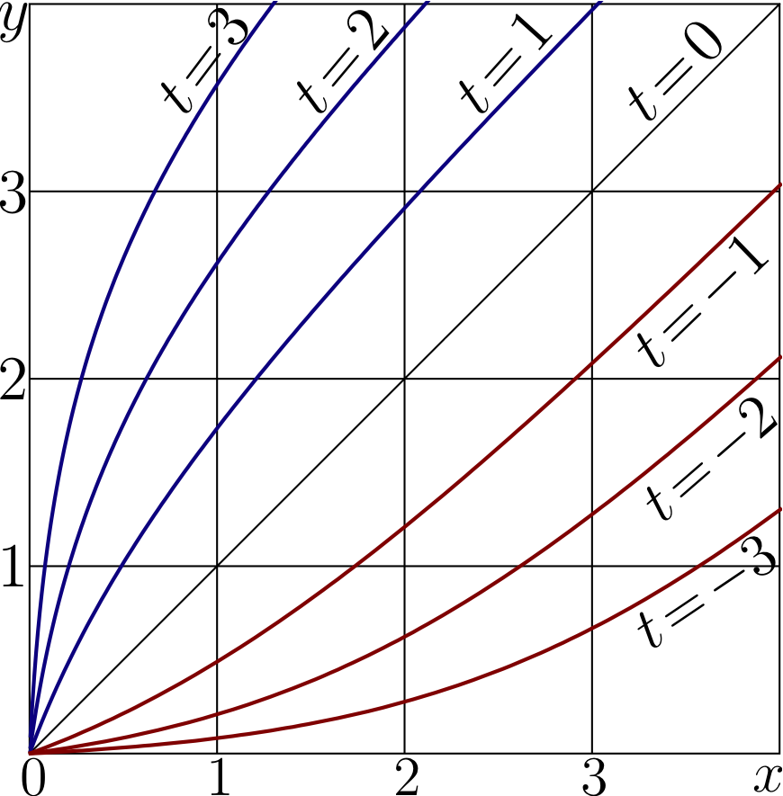 | 870 × 885 (118 KB) | Maintenance script (talk | contribs) | Importing image file |
You cannot overwrite this file.
File usage
The following page uses this file: