Difference between revisions of "File:Factorialz.jpg"
(Maintenance script uploaded "File:Factorialz.jpg": Importing image file) |
|||
| (4 intermediate revisions by 2 users not shown) | |||
| Line 1: | Line 1: | ||
| + | {{oq|Factorialz.jpg|Original file (1,706 × 1,677 pixels, file size: 932 KB, MIME type: image/jpeg)}} |
||
| − | Factorial in the complex plane. Copy from |
||
| + | |||
| + | [[Factorial]] in the complex plane. |
||
| + | |||
| + | \[ |
||
| + | u+\mathrm iv = \mathrm{Factorial}(x\!+\!\mathrm iy) |
||
| + | \] |
||
| + | |||
| + | The additional level \(u=0.8856031944\) |
||
| + | corresponds to the local minimum of [[Factorial]] of positive argument. |
||
| + | |||
| + | ==[[Superfunctions]]== |
||
| + | |||
| + | This map appears as Fig.8.3 at page 92 of book |
||
| + | «[[Superfunctions]]»<ref> |
||
| + | https://www.amazon.co.jp/Superfunctions-Non-integer-holomorphic-functions-superfunctions/dp/6202672862 Dmitrii Kouznetsov. [[Superfunctions]]: Non-integer iterates of holomorphic functions. [[Tetration]] and other [[superfunction]]s. Formulas,algorithms,tables,graphics - 2020/7/28 |
||
| + | </ref><ref>https://mizugadro.mydns.jp/BOOK/468.pdf Dmitrii Kouznetsov (2020). [[Superfunctions]]: Non-integer iterates of holomorphic functions. [[Tetration]] and other [[superfunction]]s. Formulas, algorithms, tables, graphics. Publisher: [[Lambert Academic Publishing]]. |
||
| + | </ref> |
||
| + | <br> |
||
| + | as a test of the compex double implementation of [[Factorial]], |
||
| + | but also to show its behavior in the complex plane.<br> |
||
| + | In the Book, the [[Factorial]] is interpreted as a [[Transferfunction]].<br> |
||
| + | For this function, the [[Superfunction]] |
||
| + | \(\mathrm{SuFac}\) |
||
| + | and the |
||
| + | [[Abelfunction]] |
||
| + | \(\mathrm{AuFac}=\mathrm{SuFac}^{-1}\) |
||
| + | and constructed. |
||
| + | Then the \(n\)th iterate of [[Factorial]] ie expressed as follows: |
||
| + | \[ |
||
| + | \mathrm{Factorial}^n=\mathrm{SuFac}\big(n+\mathrm{AuFac}(x)\big) |
||
| + | \] |
||
| + | In particular, at \(n!=\!1/2\), this formula expresses the [[Square root of factorial]] <ref> |
||
| + | https://link.springer.com/article/10.3103/S0027134910010029<br> |
||
| + | http://mizugadro.mydns.jp/PAPERS/2010superfae.pdf<br> |
||
| + | http://mizugadro.mydns.jp/PAPERS/2010superfar.pdf<br> |
||
| + | D.Kouznetsov, H.Trappmann. Superfunctions and square root of factorial. Moscow University Physics Bulletin, 2010, v.65, No.1, p.6-12. (Russian version: p.8-14) |
||
| + | </ref>; since century 20, it is used as LOGO of the Physics department of the [[Moscow State Univeristy]]. |
||
| + | |||
| + | ==Sitizendium== |
||
| + | Similar picture appears at |
||
http://en.citizendium.org/wiki/Image:Factorialz.jpg |
http://en.citizendium.org/wiki/Image:Factorialz.jpg |
||
| + | <!-- |
||
| + | The brown line shows the level |
||
| + | <math>u=\mu_1\approx -3.544643611</math> and corresponds to the value of the first local minimum of factorial of the real argument. |
||
| + | !--> |
||
| + | ==C++ generator of map== |
||
| + | // files [[fac.cin]], [[ado.cin]], [[conto.cin]] should be loaded |
||
| + | <pre> |
||
| + | #include <math.h> |
||
| + | #include <stdio.h> |
||
| + | #include <stdlib.h> |
||
| + | #define DB double |
||
| + | #define DO(x,y) for(x=0;x<y;x++) |
||
| + | using namespace std; |
||
| + | #include <complex> |
||
| + | typedef complex<double> z_type; |
||
| + | #define Re(x) x.real() |
||
| + | #define Im(x) x.imag() |
||
| + | #define I z_type(0.,1.) |
||
| + | #include "fac.cin" |
||
| + | //#include "sinc.cin" |
||
| + | #include "facp.cin" |
||
| + | #include "afacc.cin" |
||
| + | //#include "superfac.cin" |
||
| + | #include "conto.cin" |
||
| + | main(){ int j,k,m,n; DB x,y, p,q, t; z_type z,c,d; |
||
| − | {{attribution}} |
||
| + | int M=403,M1=M+1; |
||
| − | Description: |
||
| + | int N=401,N1=N+1; |
||
| + | DB X[M1],Y[N1], g[M1*N1],f[M1*N1], w[M1*N1]; // w is working array. |
||
| + | char v[M1*N1]; // v is working array |
||
| + | // FILE *o;o=fopen("fig2b.eps","w");ado(o,402,402); |
||
| + | FILE *o;o=fopen("facmap.eps","w");ado(o,402,402); |
||
| + | fprintf(o,"201 201 translate\n 20 20 scale\n"); |
||
| + | DO(m,212) X[m]=-8.+.04*(m); |
||
| + | X[212]=.45; |
||
| + | X[213]=.46; |
||
| + | X[214]=.47; |
||
| + | for(m=215;m<M1;m++) X[m]=-8.+.04*(m-3.); |
||
| + | DO(n,200)Y[n]=-8.+.04*n; |
||
| + | Y[200]=-.008; |
||
| + | Y[201]= .008; |
||
| + | for(n=202;n<N1;n++) Y[n]=-8.+.04*(n-1.); |
||
| + | for(m=-8;m<9;m++){if(m==0){M(m,-8.5)L(m,8.5)} else{M(m,-8)L(m,8)}} |
||
| + | for(n=-8;n<9;n++){ M( -8,n)L(8,n)} |
||
| + | fprintf(o,".008 W 0 0 0 RGB S\n"); |
||
| + | DO(m,M1)DO(n,N1){g[m*N1+n]=9999; f[m*N1+n]=9999;} |
||
| + | DO(m,M1){x=X[m]; //printf("%5.2f\n",x); |
||
| + | DO(n,N1){y=Y[n]; z=z_type(x,y); |
||
| + | // c=afacc(z); |
||
| + | c=fac(z); |
||
| + | // c=superfac(z); |
||
| + | // p=abs(c-d)/(abs(c)+abs(d)); p=-log(p)/log(10.)-1.; |
||
| + | p=Re(c);q=Im(c); |
||
| + | if(p>-9999 && p<9999 && |
||
| + | // (fabs(y)>.034 ||x>-.9 ||fabs(x-int(x))>1.e-3) && |
||
| + | q>-9999 && q<9999 //&& fabs(q)> 1.e-19 |
||
| + | ) |
||
| + | {g[m*N1+n]=p;f[m*N1+n]=q;} |
||
| + | }} |
||
| + | //fprintf(o,"1 setlinejoin 2 setlinecap\n"); p=1.8;q=.7; |
||
| + | fprintf(o,"1 setlinejoin 1 setlinecap\n"); p=1.4;q=.8; |
||
| − | In the complex <math>z</math>-plane, |
||
| + | for(m=-4;m<4;m++)for(n=2;n<10;n+=2)conto(o,f,w,v,X,Y,M,N,(m+.1*n),-q, q); fprintf(o,".025 W 0 .6 0 RGB S\n"); |
||
| − | the lines of constant <math>u=\Re(z!)</math> and |
||
| + | for(m=0;m<2;m++) for(n=2;n<10;n+=2)conto(o,g,w,v,X,Y,M,N,-(m+.1*n),-q, q); fprintf(o,".025 W .9 0 0 RGB S\n"); |
||
| − | the lines of constant <math>v=\Im(z!)</math> are shown. |
||
| + | for(m=0;m<2;m++) for(n=2;n<10;n+=2)conto(o,g,w,v,X,Y,M,N, (m+.1*n),-q, q); fprintf(o,".025 W 0 0 .9 RGB S\n"); |
||
| − | The levels |
||
| + | for(m=1;m<15;m++) conto(o,f,w,v,X,Y,M,N, (0.-m),-p,p); fprintf(o,".07 W .9 0 0 RGB S\n"); |
||
| − | <math>u= -24, -20, -16, -12, -8,-7,-6,-5,-4,-3,-2,-1,0,1,2,3,4,5,6,7,8,12,16,20,24</math> |
||
| + | for(m=1;m<15;m++) conto(o,f,w,v,X,Y,M,N, (0.+m),-p,p); fprintf(o,".07 W 0 0 .9 RGB S\n"); |
||
| − | are drown with thick black lines. |
||
| + | conto(o,f,w,v,X,Y,M,N, (0. ),-9,9); fprintf(o,".07 W .6 0 .6 RGB S\n"); |
||
| − | some of intermediate levels <math>u=</math>const are shown with thin blue lines for positive values and with thin red lines for negative values.<br> |
||
| + | for(m=-14;m<0;m++) conto(o,g,w,v,X,Y,M,N, (0.+m),-p,p); fprintf(o,".07 W 0 0 0 RGB S\n"); |
||
| − | The levels |
||
| + | m=0; conto(o,g,w,v,X,Y,M,N, (0.+m),-9,9); fprintf(o,".07 W 0 0 0 RGB S\n"); |
||
| − | <math>v= -24, -20, -16, -12, -8,-7,-6,-5,-4,-3,-2,-1</math> |
||
| + | for(m=1;m<17;m++) conto(o,g,w,v,X,Y,M,N, (0.+m),-p,p); fprintf(o,".07 W 0 0 0 RGB S\n"); |
||
| − | are shown with thick red lines.<br> |
||
| + | //#include"plofu.cin" |
||
| − | The level <math>v=0</math> |
||
| + | x=0.8856031944; |
||
| − | is shown with thick pink lines.<br> |
||
| + | conto(o,g,w,v,X,Y,M,N,0.8856031944,-p,p); fprintf(o,".02 W .5 .5 0 RGB S\n"); |
||
| − | The levels |
||
| + | /* |
||
| − | <math>v=1,2,3,4,5,6,7,8,12,16,20,24</math> |
||
| + | M(x,-8)L(x,8) fprintf(o,"0 setlinejoin 0 setlinecap 0.004 W 0 0 0 RGB S\n"); |
||
| − | are drown with thick blue lines. |
||
| + | M(x,0)L(-8.1,0) fprintf(o," .05 W 1 1 1 RGB S\n"); |
||
| − | some of intermediate levels <math>v=</math>const are shown with thin green lines.<br> |
||
| + | DO(m,23){ M(x-.4*m,0)L(x-.4*(m+.5),0);} fprintf(o,".09 W .3 .3 0 RGB S\n"); |
||
| − | The dashed blue line shows the level |
||
| + | //M(x,0)L(-8.1,0) fprintf(o,"[.19 .21]0 setdash .05 W 0 0 0 RGB S\n"); |
||
| − | <math>u=\mu_0\approx 0.88560319441</math> and corresponds to the value of the principal local minimum of the factorial of the real argument.<br> |
||
| + | // May it be, that, some printers do not interpret well the dashing ? |
||
| + | */ |
||
| + | fprintf(o,"showpage\n%c%cTrailer",'%','%'); fclose(o); |
||
| + | system("epstopdf facmap.eps"); |
||
| + | system( "open facmap.pdf"); //for LINUX |
||
| + | // getchar(); system("killall Preview");//for mac |
||
| + | } |
||
| + | </pre> |
||
| + | ==[[Latex]] generator of labels== |
||
| − | The dashed red line shows the level |
||
| + | <pre> |
||
| − | <math>u=\mu_1\approx -3.544643611</math> and corresponds to the value of the first local maximum of the factorial of the real argument. |
||
| + | \documentclass[12pt]{article} |
||
| + | \usepackage{geometry} |
||
| + | \usepackage{graphicx} |
||
| + | \usepackage{rotating} |
||
| + | \newcommand{\sx}{\scalebox} |
||
| + | \newcommand \rot {\begin{rotate}} |
||
| + | \newcommand \ero {\end{rotate}} |
||
| + | \newcommand \ing \includegraphics |
||
| + | \pagestyle{empty} |
||
| + | \topmargin -86pt |
||
| + | \oddsidemargin -96pt |
||
| + | \textwidth 1400pt |
||
| + | \textheight 1400pt |
||
| + | \paperwidth 1028pt |
||
| + | \paperheight 1010pt |
||
| + | \newcommand \ax { |
||
| + | \put( 10,342){\sx{1.4}{$y$}} |
||
| + | \put( 10,307){\sx{1.3}{$6$}} |
||
| + | \put( 10,267){\sx{1.3}{$4$}} |
||
| + | \put( 10,227){\sx{1.3}{$2$}} |
||
| + | \put( 10,187){\sx{1.3}{$0$}} |
||
| + | \put( 0,147){\sx{1.3}{$-2$}} |
||
| + | \put( 0,107){\sx{1.3}{$-4$}} |
||
| + | \put( 0, 67){\sx{1.3}{$-6$}} |
||
| + | \put( 0, 27){\sx{1.3}{$-8$}} |
||
| + | \put( 50, 18){\sx{1.3}{$-6$}} |
||
| + | \put( 90, 18){\sx{1.3}{$-4$}} |
||
| + | \put(130, 18){\sx{1.3}{$-2$}} |
||
| + | \put(178, 18){\sx{1.3}{$0$}} |
||
| + | \put(218, 18){\sx{1.3}{$2$}} |
||
| + | \put(258, 18){\sx{1.3}{$4$}} |
||
| + | \put(298, 18){\sx{1.3}{$6$}} |
||
| + | \put(334, 19){\sx{1.4}{$x$}} |
||
| + | } |
||
| + | \begin{document} |
||
| + | %\sx{1.2}{\begin{picture}(346,346) \ax |
||
| + | \sx{3}{\begin{picture}(346,346) \ax |
||
| + | \put(-20,-10){\includegraphics{facmap}} |
||
| + | \put(286,225){\rot{-7}\sx{1.6}{$v\!=\!0$}\ero} |
||
| + | \put(288,207){\rot{-5}\sx{1.6}{$u\!=\!0$}\ero} |
||
| + | \put(299,187){\sx{1.6}{$v\!=\!0$}} |
||
| + | \put(288,168){\rot{5}\sx{1.6}{$u\!=\!0$}\ero} |
||
| + | \put(286,150){\rot{7}\sx{1.6}{$v\!=\!0$}\ero} |
||
| + | \put(103,100){\rot{54}\sx{1.6}{$u\!=\!0$}\ero} |
||
| + | \put(117,100){\rot{53}\sx{1.6}{$v\!=\!0$}\ero} |
||
| + | \put(135,100){\rot{54}\sx{1.6}{$u\!=\!0$}\ero} |
||
| + | \put(152,100){\rot{54}\sx{1.6}{$v\!=\!0$}\ero} |
||
| + | \put(167, 99){\rot{50}\sx{1.6}{$u\!=\!0$}\ero} |
||
| + | \put(182, 95){\rot{41}\sx{1.6}{$v\!=\!0$}\ero} |
||
| + | \put(194, 85){\rot{39}\sx{1.6}{$u\!=\!0$}\ero} |
||
| + | \put(201, 73){\rot{35}\sx{1.6}{$v\!=\!0$}\ero} |
||
| + | \put(208, 61){\rot{33}\sx{1.6}{$u\!=\!0$}\ero} |
||
| + | \put(215, 49){\rot{28}\sx{1.6}{$v\!=\!0$}\ero} |
||
| + | \end{picture}} |
||
| + | \end{document} |
||
| + | </pre> |
||
| + | ==References== |
||
| + | {{ref}} |
||
| + | |||
| + | {{fer}} |
||
| + | ==Keywords== |
||
| + | |||
| + | «[[]]», |
||
| + | «[[Factorial]]», |
||
| + | «[[Square root of Factorial]]», |
||
| + | «[[Square root of factorial]]», |
||
| + | «[[Superfuncitons]]», |
||
| + | «[[Transferfunction]]», |
||
| + | |||
| + | [[Category:C++]] |
||
| + | [[Category:Complex map]] |
||
| + | [[Category:Book]] |
||
| + | [[Category:BookMap]] |
||
| + | [[Category:Factorial]] |
||
| + | [[Category:Latex]] |
||
| + | [[Category:Map]] |
||
[[Category:Plots of functions]] |
[[Category:Plots of functions]] |
||
[[Category:Files from CZ]] |
[[Category:Files from CZ]] |
||
| − | [[Category:Complex map]] |
||
Latest revision as of 13:16, 22 August 2025
Factorial in the complex plane.
\[ u+\mathrm iv = \mathrm{Factorial}(x\!+\!\mathrm iy) \]
The additional level \(u=0.8856031944\) corresponds to the local minimum of Factorial of positive argument.
Superfunctions
This map appears as Fig.8.3 at page 92 of book
«Superfunctions»[1][2]
as a test of the compex double implementation of Factorial,
but also to show its behavior in the complex plane.
In the Book, the Factorial is interpreted as a Transferfunction.
For this function, the Superfunction
\(\mathrm{SuFac}\)
and the
Abelfunction
\(\mathrm{AuFac}=\mathrm{SuFac}^{-1}\)
and constructed.
Then the \(n\)th iterate of Factorial ie expressed as follows:
\[
\mathrm{Factorial}^n=\mathrm{SuFac}\big(n+\mathrm{AuFac}(x)\big)
\]
In particular, at \(n!=\!1/2\), this formula expresses the Square root of factorial [3]; since century 20, it is used as LOGO of the Physics department of the Moscow State Univeristy.
Sitizendium
Similar picture appears at http://en.citizendium.org/wiki/Image:Factorialz.jpg
C++ generator of map
// files fac.cin, ado.cin, conto.cin should be loaded
 #include <math.h>
 #include <stdio.h>
 #include <stdlib.h>
 #define DB double
 #define DO(x,y) for(x=0;x<y;x++)
 using namespace std;
 #include <complex>
 typedef complex<double> z_type;
 #define Re(x) x.real()
 #define Im(x) x.imag()
 #define I z_type(0.,1.)
 #include "fac.cin"
 //#include "sinc.cin"
 #include "facp.cin"
 #include "afacc.cin"
 //#include "superfac.cin"
 #include "conto.cin"

 main(){ int j,k,m,n; DB x,y, p,q, t; z_type z,c,d;
   int M=403,M1=M+1;
   int N=401,N1=N+1;
 DB X[M1],Y[N1], g[M1*N1],f[M1*N1], w[M1*N1]; // w is working array.
 char v[M1*N1]; // v is working array
 // FILE *o;o=fopen("fig2b.eps","w");ado(o,402,402);
 FILE *o;o=fopen("facmap.eps","w");ado(o,402,402);
 fprintf(o,"201 201 translate\n 20 20 scale\n");
 DO(m,212) X[m]=-8.+.04*(m);
    X[212]=.45;
    X[213]=.46;
    X[214]=.47;
 for(m=215;m<M1;m++) X[m]=-8.+.04*(m-3.);
 DO(n,200)Y[n]=-8.+.04*n;
         Y[200]=-.008;
         Y[201]= .008;
 for(n=202;n<N1;n++) Y[n]=-8.+.04*(n-1.);
 for(m=-8;m<9;m++){if(m==0){M(m,-8.5)L(m,8.5)} else{M(m,-8)L(m,8)}}
 for(n=-8;n<9;n++){	M(  -8,n)L(8,n)}
 fprintf(o,".008 W 0 0 0 RGB S\n");
 DO(m,M1)DO(n,N1){g[m*N1+n]=9999; f[m*N1+n]=9999;}
 DO(m,M1){x=X[m]; //printf("%5.2f\n",x);
 DO(n,N1){y=Y[n]; z=z_type(x,y);
 //	c=afacc(z);
 	c=fac(z);
 //	c=superfac(z);
 //	p=abs(c-d)/(abs(c)+abs(d));  p=-log(p)/log(10.)-1.;
 	p=Re(c);q=Im(c);
 	if(p>-9999 && p<9999 &&
 //	  (fabs(y)>.034 ||x>-.9 ||fabs(x-int(x))>1.e-3) &&
 	   q>-9999 && q<9999 //&& fabs(q)> 1.e-19
 	)
 	{g[m*N1+n]=p;f[m*N1+n]=q;}
 			}}
 //fprintf(o,"1 setlinejoin 2 setlinecap\n"); p=1.8;q=.7;

 fprintf(o,"1 setlinejoin 1 setlinecap\n"); p=1.4;q=.8;
 for(m=-4;m<4;m++)for(n=2;n<10;n+=2)conto(o,f,w,v,X,Y,M,N,(m+.1*n),-q, q); fprintf(o,".025 W 0 .6 0 RGB S\n");
 for(m=0;m<2;m++) for(n=2;n<10;n+=2)conto(o,g,w,v,X,Y,M,N,-(m+.1*n),-q, q); fprintf(o,".025 W .9 0 0 RGB S\n");
 for(m=0;m<2;m++) for(n=2;n<10;n+=2)conto(o,g,w,v,X,Y,M,N, (m+.1*n),-q, q); fprintf(o,".025 W 0 0 .9 RGB S\n");
 for(m=1;m<15;m++)  conto(o,f,w,v,X,Y,M,N, (0.-m),-p,p); fprintf(o,".07 W .9 0 0 RGB S\n");
 for(m=1;m<15;m++)  conto(o,f,w,v,X,Y,M,N, (0.+m),-p,p); fprintf(o,".07 W 0 0 .9 RGB S\n");
                  conto(o,f,w,v,X,Y,M,N, (0.  ),-9,9); fprintf(o,".07 W .6 0 .6 RGB S\n");
 for(m=-14;m<0;m++) conto(o,g,w,v,X,Y,M,N, (0.+m),-p,p); fprintf(o,".07 W 0 0 0 RGB S\n");
           m=0;     conto(o,g,w,v,X,Y,M,N, (0.+m),-9,9); fprintf(o,".07 W 0 0 0 RGB S\n");
 for(m=1;m<17;m++) conto(o,g,w,v,X,Y,M,N, (0.+m),-p,p); fprintf(o,".07 W 0 0 0 RGB S\n");
//#include"plofu.cin"
 x=0.8856031944;
 conto(o,g,w,v,X,Y,M,N,0.8856031944,-p,p); fprintf(o,".02 W .5 .5 0 RGB S\n");
/*
 M(x,-8)L(x,8) fprintf(o,"0 setlinejoin 0 setlinecap 0.004 W 0 0 0 RGB S\n");
 M(x,0)L(-8.1,0) fprintf(o,"                   .05 W  1 1 1 RGB S\n");
 DO(m,23){ M(x-.4*m,0)L(x-.4*(m+.5),0);} fprintf(o,".09 W  .3 .3 0 RGB S\n");
 //M(x,0)L(-8.1,0) fprintf(o,"[.19 .21]0 setdash .05 W  0 0 0 RGB S\n");
 // May it be, that, some printers do not interpret well the dashing ?
*/
 fprintf(o,"showpage\n%c%cTrailer",'%','%'); fclose(o);
 	system("epstopdf facmap.eps");
 	system(    "open facmap.pdf");	//for LINUX
 //	getchar(); system("killall Preview");//for mac
 }
Latex generator of labels
\documentclass[12pt]{article}
\usepackage{geometry}
\usepackage{graphicx}
\usepackage{rotating}
\newcommand{\sx}{\scalebox}
\newcommand \rot {\begin{rotate}}
\newcommand \ero {\end{rotate}}
\newcommand \ing \includegraphics
\pagestyle{empty}
\topmargin -86pt
\oddsidemargin -96pt
\textwidth 1400pt
\textheight 1400pt
\paperwidth 1028pt
\paperheight 1010pt
\newcommand \ax {
\put( 10,342){\sx{1.4}{$y$}}
\put( 10,307){\sx{1.3}{$6$}}
\put( 10,267){\sx{1.3}{$4$}}
\put( 10,227){\sx{1.3}{$2$}}
\put( 10,187){\sx{1.3}{$0$}}
\put(  0,147){\sx{1.3}{$-2$}}
\put(  0,107){\sx{1.3}{$-4$}}
\put(  0, 67){\sx{1.3}{$-6$}}
\put(  0, 27){\sx{1.3}{$-8$}}
\put( 50, 18){\sx{1.3}{$-6$}}
\put( 90, 18){\sx{1.3}{$-4$}}
\put(130, 18){\sx{1.3}{$-2$}}
\put(178, 18){\sx{1.3}{$0$}}
\put(218, 18){\sx{1.3}{$2$}}
\put(258, 18){\sx{1.3}{$4$}}
\put(298, 18){\sx{1.3}{$6$}}
\put(334, 19){\sx{1.4}{$x$}}
}

\begin{document}
%\sx{1.2}{\begin{picture}(346,346) \ax
\sx{3}{\begin{picture}(346,346) \ax
\put(-20,-10){\includegraphics{facmap}}
\put(286,225){\rot{-7}\sx{1.6}{$v\!=\!0$}\ero}
\put(288,207){\rot{-5}\sx{1.6}{$u\!=\!0$}\ero}
\put(299,187){\sx{1.6}{$v\!=\!0$}}
\put(288,168){\rot{5}\sx{1.6}{$u\!=\!0$}\ero}
\put(286,150){\rot{7}\sx{1.6}{$v\!=\!0$}\ero}
\put(103,100){\rot{54}\sx{1.6}{$u\!=\!0$}\ero}
\put(117,100){\rot{53}\sx{1.6}{$v\!=\!0$}\ero}
\put(135,100){\rot{54}\sx{1.6}{$u\!=\!0$}\ero}
\put(152,100){\rot{54}\sx{1.6}{$v\!=\!0$}\ero}
\put(167, 99){\rot{50}\sx{1.6}{$u\!=\!0$}\ero}
\put(182, 95){\rot{41}\sx{1.6}{$v\!=\!0$}\ero}
\put(194, 85){\rot{39}\sx{1.6}{$u\!=\!0$}\ero}
\put(201, 73){\rot{35}\sx{1.6}{$v\!=\!0$}\ero}
\put(208, 61){\rot{33}\sx{1.6}{$u\!=\!0$}\ero}
\put(215, 49){\rot{28}\sx{1.6}{$v\!=\!0$}\ero}
\end{picture}}
\end{document}
References
- ↑ https://www.amazon.co.jp/Superfunctions-Non-integer-holomorphic-functions-superfunctions/dp/6202672862 Dmitrii Kouznetsov. Superfunctions: Non-integer iterates of holomorphic functions. Tetration and other superfunctions. Formulas,algorithms,tables,graphics - 2020/7/28
- ↑ https://mizugadro.mydns.jp/BOOK/468.pdf Dmitrii Kouznetsov (2020). Superfunctions: Non-integer iterates of holomorphic functions. Tetration and other superfunctions. Formulas, algorithms, tables, graphics. Publisher: Lambert Academic Publishing.
- ↑
https://link.springer.com/article/10.3103/S0027134910010029
http://mizugadro.mydns.jp/PAPERS/2010superfae.pdf
http://mizugadro.mydns.jp/PAPERS/2010superfar.pdf
D.Kouznetsov, H.Trappmann. Superfunctions and square root of factorial. Moscow University Physics Bulletin, 2010, v.65, No.1, p.6-12. (Russian version: p.8-14)
Keywords
«[[]]», «Factorial», «Square root of Factorial», «Square root of factorial», «Superfuncitons», «Transferfunction»,
File history
Click on a date/time to view the file as it appeared at that time.
| Date/Time | Thumbnail | Dimensions | User | Comment | |
|---|---|---|---|---|---|
| current | 13:10, 22 August 2025 |  | 1,706 × 1,677 (932 KB) | T (talk | contribs) | closer to that in book Superfunctions |
| 17:50, 20 June 2013 | 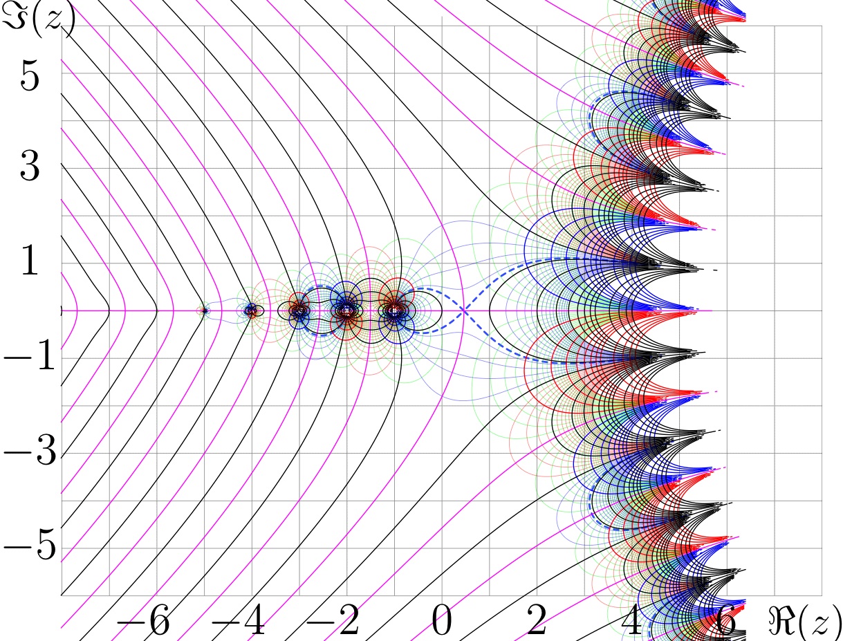 | 1,219 × 927 (479 KB) | Maintenance script (talk | contribs) | Importing image file |
You cannot overwrite this file.
File usage
The following page uses this file: