Search results

Create the page "Explicit plots" on this wiki! See also the search results found.

• SuperFactorial
  </ref>. The regular iteration gives the explicit proof of existence, while the requirements on the behavior at zero and the
  18 KB (2,278 words) - 00:03, 29 February 2024
• LogisticSequence
  For various values of \(s\), the explicit plots of LogisticSequence are shown in two figures at right. Below, the [[complex
  7 KB (886 words) - 18:26, 30 July 2019
• Efjh.cin
  ...e stored as [[efjh.cin]] in order to compile the generators of pictures ([[explicit plot]]s and/or the [[complex map]]s) of the [[LogisticSequence]]. Sorry for
  3 KB (364 words) - 07:00, 1 December 2018
• Logistic operator
  The [[explicit plot]]s of the Logistic operator for \(s\!=\!3\), \(s\!=\!4\) and \(s\!=\!5 ...ient algorithms for the evaluation are supplied. With these functions, the explicit plot of some iterations of the logistic operators are
  6 KB (817 words) - 19:54, 5 August 2020
• Power function
  For \(a\!=\!2\), the explicit plots of these two functions are shown in Fig.3.
  15 KB (2,495 words) - 18:43, 30 July 2019

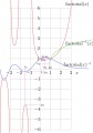
• File:FactoReal.jpg [[Category:plots of functions]] [[Category:Explicit plot]] (915 × 1,310 (141 KB)) - 08:35, 1 December 2018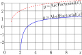

• File:AbelFactorialR.png [[Category:Explicit plots]] (1,060 × 705 (34 KB)) - 09:39, 21 June 2013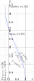

• File:AsincplotT500.png Explicit plot of functions [[ArcSinc]] (thick blue curve) and [[ArcCosc]] (thin red [[Category:Explicit plots]] (843 × 2,014 (184 KB)) - 09:41, 21 June 2013

• File:Ater01.png [[Category:Explicit plots]] (1,192 × 1,096 (174 KB)) - 08:30, 1 December 2018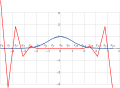

• File:FFTexample16T.png [[Category:Explicit plots]] (2,101 × 1,536 (155 KB)) - 09:39, 21 June 2013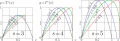

• File:Logi1a345T300.png [[Explicit plot]]s of various iterations of the [[Logistic operator]] with various val (1,636 × 565 (184 KB)) - 08:41, 1 December 2018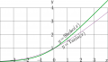

• File:ShokotaniaT.png [[Explicit plot]]s of the [[Shoko function]] (thick curve) and the [[Tania function]] [[Category:Explicit plot]] (1,669 × 955 (119 KB)) - 08:51, 1 December 2018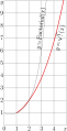

• File:SquareRootOfFactorial.png [[Category:Explicit plots]] (538 × 1,050 (34 KB)) - 09:39, 21 June 2013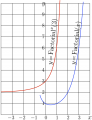

• File:Superfactorea500.png # [[Superfactoreal.cc]] , that plots the curves as superfactoreal.pdf ...ecial implementation for the real values of the argument; so, for the real plots, the real part of the output is used. (575 × 748 (50 KB)) - 00:06, 29 February 2024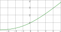

• File:TaniaPlot.png Explicit plot of the [[Tania function]], $y=\mathrm{Tania}(x)$. [[Category:Explicit plots]] (807 × 424 (16 KB)) - 09:39, 21 June 2013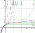

• File:Tetreal10bx10d.png [[Category:Explicit plot]] [[Category:Real-real plots]] (2,192 × 2,026 (436 KB)) - 13:56, 5 August 2020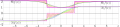

• File:TetSheldonImaT.png [[Category:Explicit plots]] (4,359 × 980 (598 KB)) - 09:40, 21 June 2013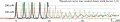

• File:TodaShow.png [[Category:Explicit plots]] (1,707 × 317 (155 KB)) - 09:39, 21 June 2013

• File:YulyPlot.png Explicit plot of [[Yylya function]], [[Category:Explicit plots]] (1,048 × 2,546 (153 KB)) - 09:39, 21 June 2013

• Abelpower
  For \(a\!=\!2\), the explicit plots of these two functions are shown in figure at top. ...elfunction]]s. Superpower and abelpower are easy to evaluate through their explicit representations; so, the precision of some general method of evaluation is
  3 KB (470 words) - 18:47, 30 July 2019

View (previous 20 | next 20) (20 | 50 | 100 | 250 | 500)