Search results
Create the page "Linear function" on this wiki! See also the search results found.
Page title matches
- #redirect[[Linear fuction]]27 bytes (3 words) - 12:58, 6 September 2013
Page text matches
- ...tself or to another space, and also the graphical representation of such a function. Such a representation is called '''map'''. ...e. Similarly, the geophysicists use some maps without to know what kind of function (it is called "projection") relates the position of a point on the surface14 KB (2,275 words) - 18:25, 30 July 2019
- it is [[holomorpic function]] in the range that includes the real axis. ...his equation, the [[tetration]] \(\mathrm{tet}\) appears as the [[transfer function]].7 KB (1,090 words) - 18:49, 30 July 2019
- ...of the statistical significance of a “second” peak at the correlation function, using the Poissonian model of random (independent) distribution, that can ...ture for years 1989-2020, fit them with linear function and with quadratic function, and check, if the raise of mean temperature accelerates during 30 years si100 KB (14,715 words) - 16:21, 31 October 2021
- ...or '''regular iterate''' refer to the [[fractional iterate]] a holomorphic function that is holomorphic in vicinity it its fixed point A [[fractional iterate]] $\phi$ of an analytic function $f$ at fixpoint $a$ is called regular, iff $\phi$ is analytic at $a$ or has20 KB (3,010 words) - 18:11, 11 June 2022
- Function \(F(M,\vec y)\) means some statistical procedure that tries to reveal any p ...rities/peculiarities in it) is to guess a number representable as a linear function of \(X\) with rational coefficients. The set of such numbers has measure ze2 KB (368 words) - 18:27, 30 July 2019
- ...pulses ([[Keller function]]) and for the continuous-wave operation ([[Doya function]])]] '''Transfer function''' \(h\) is expression of the state of the system in terms of its state at11 KB (1,644 words) - 06:33, 20 July 2020
- For a given function \(f\), the '''fixed point''' is solution \(L\) of equation In the simple case, \(f\) is just [[holomorphic function]] of a single variable; then \(L\) is assumed to be a [[complex number]].4 KB (574 words) - 18:26, 30 July 2019
- ...|right|thumb| Comparison of [[Tania function]] (thin curve) to the [[Shoka function]] (thick curve) for real values of the argument]] '''Tania function''' is solution \(f\!=\!\mathrm{Tania}\) of equation27 KB (4,071 words) - 18:29, 16 July 2020
- '''Fourier transform''' is linear integral transform with the exponential [[kernel]]. Let some complex–valued function \(A\) be defined for real values of the argument, id est,11 KB (1,501 words) - 18:44, 30 July 2019
- For a given function \(T\), called [[transfer function]], the holomorphic solution \(F\) of [[Transfer equation]] The inverse function, id est, \(G=F^{-1}\) is called [[Abel function]] with respect to \(T\); it satisfies the [[Abel equation]]11 KB (1,565 words) - 18:26, 30 July 2019
- ...bservable [[physical quantities]] as [[Hermitian operator]]s acting on the linear space of [[vector of state|vectors of state]]. ...m]] is characterized with an element \(\psi\) of the [[linear space]]; any linear combinaiton of the states of a physical system is also interpreted as the s7 KB (1,006 words) - 18:26, 30 July 2019
- ...ерация]]) is function, expressed as repetition of another (iterated) function, that may be called [[iterand]]. Any function by itself is considered as its first iteration.14 KB (2,203 words) - 06:36, 20 July 2020
- Function \(\mathrm {tet}(z)\) is holomorphic in the whole complex plane except the l where \(\eta\) is holomorphic periodic function with period unity,14 KB (1,972 words) - 02:22, 27 June 2020
- The transform \(g\) of a function \(f\) is defined with expression The Fourier transform can be used for the filtering of the function. An example of such a filtering is suggested below.6 KB (954 words) - 18:27, 30 July 2019
- '''Acosc1''' is the holomorphic continuation of function [[ArcCosc]] behind the cut line along the negative part of the real axis. In the text, this function appears with names ArcCosc1, or acosc1;6 KB (896 words) - 18:26, 30 July 2019
- at order \(\nu\) is operator that converts function \(f\) to function \(g=\mathrm{BesselTransform}_\nu(f)\) such that where [[BesselJ]]\(_\nu\) is the [[Bessel function]], and8 KB (1,183 words) - 10:21, 20 July 2020
- '''Cylindric function''' (or cylinder finction or cylindrical function) is class of special functions \(f\) satisfying equation http://encyclopedia2.thefreedictionary.com/Cylindrical+Function3 KB (388 words) - 18:26, 30 July 2019
- where \(f\) is smooth function of real positive argument. One may extend \(f\) to the negative values of t At large \(N\), smoothness and quick decay at infinity is assumed for function \(f\).3 KB (421 words) - 18:26, 30 July 2019
- ...urier]] operator transforms a function \(F\) of non–negative argument to function \(G\) in the following way: Let function \(F\) be smooth and quickly decay at infinity. Then, the transform of \(F\)10 KB (1,447 words) - 18:27, 30 July 2019
- \(T\) is assumed to be [[scalar] function of scalar argument. but the smoothness of function(s) \(q\) is assumed.10 KB (1,317 words) - 18:25, 30 July 2019
- ...rete cosine transform is a [[linear]], invertible [[function (mathematics)|function]] ''F'' : '''R'''<sup>''N''</sup> <tt>-></tt> '''R'''<sup>''N''</sup> or10 KB (1,689 words) - 18:26, 30 July 2019
- The example of the C++ call below calculates the expansion of function Let \(F\) be smooth even function quickly decaying at infinity; let \(N\) be large natural number.5 KB (682 words) - 18:27, 30 July 2019
- [[File:ShokopPlotAT.png|400px|thumb|[[Shoko function]] and two its asimptitics]] [[Shoko function]] describes the growth of the [[fluence]] of pulse of light in the homogene10 KB (1,507 words) - 18:25, 30 July 2019
- [[Trappmann function]] is defined with ...re elementary function. The Trappmann function is example of [[holomorphic function]] without [[fixed point]]s, suggested in year 2011 by [[Henryk Trappmann]]9 KB (1,320 words) - 11:38, 20 July 2020
- ArcTra is inverse of the [[Trappmann function]]; \(\mathrm{ArcTra}=\mathrm{tra}^{-1}\), where [[ArcTra]] can be expressed through the [[Tania function]] as follows:10 KB (1,442 words) - 18:47, 30 July 2019
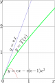
File:DoyaplotTc.png [[Doya function]] with parameter unity of real argument, $y=T(x)=\mathrm{Doya}_1(x)$ The linear approximation in vicinity of zero $y=T'(0) x =\mathrm e x~$(881 × 1,325 (95 KB)) - 09:43, 21 June 2013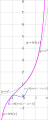
File:TetPlotU.png ...aphic of tetration $y\!=\!\mathrm{tet}(x)$ looks similar to that of linear function ...tetration $y\!=\!\mathrm{tet}(x)$ looks similar to that of the exponential function $y\!=\!\exp(x)$.(838 × 2,088 (124 KB)) - 08:53, 1 December 2018- ...t is assumed that the inverse function \(Q=P^{-1}\) exists. Then, for some function \(f\), its conjugate \(g\) is expressed with ..., the operations \(P\) and \(f\) commute, and \(P\) can be "drawn through" function \(f\), for example,6 KB (921 words) - 18:46, 30 July 2019
- ...rate_of_linear_fraction]] (or [[iteration of linnet friaction]]) refers to function [[Iterate]] of a [[linear fraction]] can be expressed with also some linear fraction. This article describes this expression.13 KB (2,088 words) - 06:43, 20 July 2020
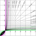
File:Fracit20t150.jpg [[Iterate of linear fraction]]; [[Category:Elementary function]](1,466 × 1,466 (463 KB)) - 08:36, 1 December 2018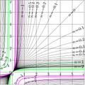
File:Fracit10t150.jpg [[Iterate of linear fraction]]; [[Category:Elementary function]](1,466 × 1,466 (564 KB)) - 08:36, 1 December 2018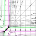
File:Fracit05t150.jpg [[Iterate of linear fraction]]; [[Category:Elementary function]](1,466 × 1,466 (441 KB)) - 08:36, 1 December 2018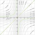
File:Frac1zt.jpg [[Iterate]]s of function $T(z)=-1/z$ The non-integer iterates of function $T$ are evaluated using the superfunction(2,089 × 2,089 (734 KB)) - 08:36, 1 December 2018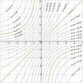
File:Frac2zt.jpg [[Iteration]] of function $T(z)=-4/z$. [[Category:Iterate of linear fraction]](2,089 × 2,089 (716 KB)) - 21:47, 29 August 2013- [[File:F1xmapT.jpg|300px|thumb|[[Complex map|Map]] of function \(T\) by (1) at \(u\!=\!0\), \(v\!=\!-1\), \(w\!=0\)]] [[Linear fraction]] is meromorphic function that can be expressed with5 KB (830 words) - 18:44, 30 July 2019
- [[Linear function]] is function that can be represented in form [[Superfunction]] \(F\) for the linear function \(T\) by (1) can be written as follows:2 KB (234 words) - 18:43, 30 July 2019
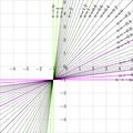
File:Itelin125T.jpg Iterates of the linear function [[Category:Linear function]](2,088 × 2,088 (893 KB)) - 08:38, 1 December 2018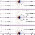
File:Fz2z1mapT.jpg [[Complex map]] of function [[Category:Linear fraction]](4,175 × 4,175 (1.57 MB)) - 08:36, 1 December 2018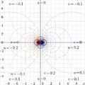
File:Gz2z1mapT.jpg [[Complex map]] of function [[Category:Abel function]](4,175 × 4,175 (1.67 MB)) - 08:37, 1 December 2018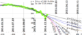
File:2014.12.26rubleDollar.png with function daju24 defined below in C++: \begin{verbatim} \rm Linear &227.323 - 0.583872 x &\! 10.52733 &\! 13.15973\\(1,502 × 651 (246 KB)) - 08:26, 1 December 2018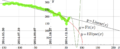
File:2014.12.29rubleDollar.png The straight black line represents the linear approximation of the data, $y=\mathrm{Linear}(x)=227.499 - 0.581655 x$(1,502 × 610 (142 KB)) - 08:26, 1 December 2018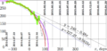
File:2014.12.31rudo.png ==Linear approximations== The thin straight lines show the two linear approximations:(1,452 × 684 (190 KB)) - 08:26, 1 December 2018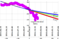
File:2014rubleDollar2param.png 10 red lines represent the linear approximations, for $M-10\le m \le M$; in such a way, for function $f=L$, 10 curves are plotted, and these curve form the red strip.(1,527 × 1,004 (232 KB)) - 08:26, 1 December 2018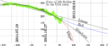
File:2014specula.png ==Linear approximation== The black straight line shows the linear approximation,(1,502 × 651 (177 KB)) - 08:26, 1 December 2018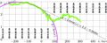
File:2015ruble2.jpg The pink arc shows function $y=\mathrm{Arc}(x)=.01\sqrt{(123-x)(471+x)}$ The black line shows the linear approximation, $y=2.4-0.0048x$(1,726 × 709 (248 KB)) - 08:26, 1 December 2018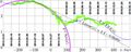
File:2015ruble3.jpg The pink arc shows function $y=\mathrm{Arc}(x)=.01\sqrt{(123-x)(471+x)} ~$ The black line shows the linear approximation, $y=2.4-0.0048x$(1,726 × 684 (266 KB)) - 08:26, 1 December 2018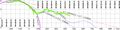
File:2016ruble1.jpg The pink arc shows function $y=\mathrm{Arc}(x)=.01\sqrt{(123-x)(471+x)} ~$ The black line shows the linear approximation, $y=2.4-0.0048x$(2,764 × 684 (414 KB)) - 08:27, 1 December 2018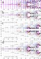
File:Analuxp01t400.jpg In this case, it is easier to guess the asymptotic behaviour of the function (last picture, d) from its primitive fit (picture b). ===a: Linear approximation by Gusmad===(2,083 × 3,011 (1.67 MB)) - 08:29, 1 December 2018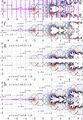
File:Analuxp01u400.jpg ===e: Linear approximation by Gusmad=== This is approximation, linear in the ramge $-1 < \Re(z) \le 0$(2,083 × 3,011 (1.72 MB)) - 08:29, 1 December 2018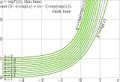
File:Exp1exp2t.jpg The corresponding linear combinations of the first and the second iterates of the exponent are defin D.Kouznetsov. Superexponential as special function. [[Vladikavkaz Mathematical Journal]], 2010, v.12, issue 2, p.31-45.(1,278 × 875 (296 KB)) - 08:35, 1 December 2018


